Lab 3
Data wrangling (tidyr)
So far we’ve mostly dealt with data that’s neatly organized into a format that is easy for us to manipulate with things like filter() and mutate(). In general, long format makes things easier: one row for every trial for each subject.Often data will not be organized so neatly from the get-go and you will have to do some serious data wrangling to get it into the format you want. In particular, you’ll see that Amazon Mechanical Turk output is often in wide format. For these purposes you will need to know functions like spread(), gather(), and separate().
First let’s set up our workspace and read in some data files. These contain data from a study of lexical decision latencies in beginning readers (8 year-old Dutch children). This is available as the beginningReaders dataset from languageR but here I’ve split it up into separate datasets so that we can see how we could put it back together.
library(tidyverse)

data_source <- "http://web.mit.edu/psycholinglab/data/"
word_data <- read_csv(file.path(data_source, "word_data.csv"))
subject_data <- read_csv(file.path(data_source, "subject_data.csv"))
logRT_data <- read_csv(file.path(data_source, "logRT_data.csv"))
Let’s look at these data:
glimpse(word_data)## Observations: 736
## Variables: 3
## $ Word <chr> "avontuur", "baden", "balkon", "band", "barsten", "beek...
## $ metric <chr> "OrthLength", "OrthLength", "OrthLength", "OrthLength",...
## $ v <dbl> 8, 5, 6, 4, 7, 4, 5, 5, 5, 6, 7, 7, 5, 6, 9, 4, 5, 5, 4...Here we see that we have a list of words and a series of metrics for each word with an associated value.
glimpse(subject_data)## Observations: 59
## Variables: 2
## $ Subject <chr> "S28", "S40", "S37", "S65", "S54", "S43", "S34", ...
## $ ReadingScore <int> 39, 34, 61, 66, 41, 23, 28, 60, 87, 39, 49, 86, 5...Here we have a reading score for each subject.
glimpse(logRT_data)## Observations: 59
## Variables: 185
## $ Subject <chr> "S10", "S12", "S13", "S14", "S15", "S16", "S18", "...
## $ avontuur <chr> "407t8.05706068196577", "155t7.66058546170326", "3...
## $ baden <chr> "398t7.93164402145431", "311t7.52940645783701", "1...
## $ balkon <chr> "133t6.83840520084734", "386t7.60738142563979", NA...
## $ band <chr> "98t7.20414929203594", "108t6.71901315438526", "41...
## $ barsten <chr> "237t7.71601526664259", "20t7.07665381544395", "50...
## $ beek <chr> "363t7.4667994750186", "394t7.36707705988101", "86...
## $ beker <chr> "186t7.46393660446893", "272t6.69703424766648", "2...
## $ beton <chr> NA, NA, "283t7.28207365809346", "511t7.51370924783...
## $ beven <chr> "38t6.90575327631146", "99t7.01031186730723", "425...
## $ bieden <chr> "66t7.85321638815607", NA, NA, "470t7.266827347520...
## $ blaffen <chr> "336t6.94408720822953", "261t7.05444965813294", "2...
## $ blinken <chr> "343t7.77275271646874", "69t6.97728134163075", "46...
## $ bocht <chr> "283t7.45818615734049", "186t6.91274282049318", "3...
## $ bonzen <chr> NA, NA, "262t6.92067150424868", NA, NA, "265t7.711...
## $ boodschap <chr> "111t7.05272104923232", "278t7.4448332738922", "22...
## $ bord <chr> NA, "91t7.15148546390474", "436t8.00670084544037",...
## $ broek <chr> "311t7.7393592026891", "427t7.7985230536252", "43t...
## $ broer <chr> "97t6.5694814204143", "326t7.31521838975297", "168...
## $ brok <chr> "476t7.67089483136212", "147t6.71052310945243", "3...
## $ brullen <chr> "448t7.1785454837637", "62t6.85751406254539", "469...
## $ buit <chr> NA, "88t6.5410299991899", "439t6.03548143252476", ...
## $ bukken <chr> "434t7.81116338502528", "315t6.8134445995109", "17...
## $ cent <chr> "413t7.01571242048723", "393t7.29776828253138", "8...
## $ deken <chr> NA, "40t6.78105762593618", "490t6.79346613258001",...
## $ douche <chr> "421t6.5510803350434", "292t7.03878354138854", "20...
## $ durven <chr> "256t7.82204400818562", "31t6.77878489768518", "49...
## $ dwingen <chr> "130t7.3864708488299", "115t6.76734312526539", "40...
## $ echo <chr> "270t7.25700270709207", "243t6.93537044601511", "2...
## $ emmer <chr> "224t7.10002716662926", "233t6.94119005506837", NA...
## $ flitsen <chr> "122t7.46164039220858", "15t7.00397413672268", "51...
## $ fluisteren <chr> "264t7.89989532313973", "312t7.37963215260955", "1...
## $ fruit <chr> "177t7.53315880745556", "1t6.99576615630485", "526...
## $ gapen <chr> "328t8.01002752848173", "300t7.14677217945264", "1...
## $ garage <chr> "141t7.12528309151071", "4t6.98378996525813", "523...
## $ giechelen <chr> "6t7.94944442025063", "89t6.95177216439891", "438t...
## $ gieten <chr> NA, "25t7.01121398735037", "503t5.97888576490112",...
## $ gillen <chr> "268t7.30518821539304", "54t7.23417717974985", "47...
## $ glinsteren <chr> "378t7.91717198884578", "335t6.98933526597456", "1...
## $ gloeien <chr> "154t6.79570577517351", "336t7.028201432058", "158...
## $ gluren <chr> "307t7.21744343169653", "414t8.22067217029725", "6...
## $ graan <chr> "425t6.49072353450251", "412t7.10824413973154", "6...
## $ grap <chr> "342t7.90285719128058", "344t7.69893619981345", "1...
## $ grijns <chr> "32t7.20191631753163", "220t7.04403289727469", "28...
## $ grijnzen <chr> "409t7.42714413340862", "56t7.13169851046691", "47...
## $ grinniken <chr> "164t7.42892719480227", "102t7.34794382314869", "4...
## $ groeten <chr> "408t7.26052259808985", "388t7.17011954344963", "9...
## $ grommen <chr> "430t7.1770187659099", "283t7.0352685992811", "219...
## $ grot <chr> "346t7.65633716643018", "173t6.97541392745595", NA...
## $ hijgen <chr> "317t7.4277388405329", "439t7.02731451403978", "28...
## $ hijsen <chr> NA, "227t7.61381868480863", "274t7.646353722446", ...
## $ horizon <chr> NA, "370t7.44073370738926", "114t7.40367029001237"...
## $ horloge <chr> "16t7.05531284333975", "223t7.12929754892937", "27...
## $ insekt <chr> "85t7.24351297466548", NA, NA, "454t7.542213463193...
## $ jagen <chr> "7t7.19142933003638", "119t6.71780469502369", "399...
## $ juichen <chr> "11t7.06646697013696", "60t6.89264164117209", NA, ...
## $ kanon <chr> "87t7.03878354138854", "73t6.96602418710611", "460...
## $ karton <chr> "351t7.59890045687141", "9t6.78558764500793", "519...
## $ karwei <chr> "394t8.0734029689864", "2t7.20191631753163", "525t...
## $ kerel <chr> "376t7.44600149832412", "383t7.29233717617388", NA...
## $ ketel <chr> "115t7.55485852104068", "327t6.85329909318608", "1...
## $ kilo <chr> "145t7.3362856600213", "437t7.15851399732932", "30...
## $ kin <chr> "216t7.29301767977278", "438t7.34148385236316", "2...
## $ klagen <chr> "211t7.34794382314869", "152t7.59034694560257", "3...
## $ klant <chr> "309t6.78445706263764", "43t7.07918439460967", "48...
## $ knagen <chr> "200t7.13966033596492", "63t7.14834574390007", "46...
## $ kneden <chr> "126t8.24222989137223", NA, NA, "409t8.23536064375...
## $ knielen <chr> "106t7.89020821310996", "347t7.30720231476474", NA...
## $ knipperen <chr> "422t7.58933582317062", NA, "256t6.62671774924902"...
## $ knol <chr> "269t7.64778604544093", "110t6.89972310728487", "4...
## $ koffer <chr> "64t7.36707705988101", "146t6.67329796776765", "36...
## $ koning <chr> "72t6.84374994900622", "41t6.54678541076052", NA, ...
## $ koren <chr> NA, "279t7.11963563801764", "223t7.95014988765202"...
## $ korst <chr> "301t6.98933526597456", "318t7.10987946307227", "1...
## $ kraag <chr> "101t6.95654544315157", "101t7.30451594646016", "4...
## $ kreunen <chr> "132t6.84374994900622", "451t7.3460102099133", NA,...
## $ krijsen <chr> "423t7.8659554139335", "179t7.2848209125686", "326...
## $ krimpen <chr> "12t7.19893124068817", "458t7.52240023138712", "4t...
## $ kudde <chr> NA, "74t6.72142570079064", "459t5.83188247728352",...
## $ kus <chr> "26t6.86589107488344", "323t6.8265452235566", "171...
## $ ladder <chr> "272t7.85360481309784", "17t7.25276241805319", "51...
## $ laden <chr> NA, "324t7.19443685110033", "170t7.55118686729615"...
## $ lawaai <chr> "419t7.89580837708318", "374t7.64156444126097", "1...
## $ leunen <chr> "440t7.25770767716004", "289t7.36707705988101", "2...
## $ liegen <chr> "180t7.19142933003638", "109t7.27170370688737", NA...
## $ lijden <chr> "48t7.61085279039525", "143t6.9037472575846", "366...
## $ liter <chr> "33t6.97260625130175", "210t7.03085747611612", NA,...
## $ loeren <chr> "468t7.49387388678356", "240t7.01750614294126", "2...
## $ manier <chr> "286t6.92853781816467", "317t7.13727843726039", "1...
## $ matras <chr> "19t7.29979736675816", "429t6.88959130835447", "41...
## $ matroos <chr> "444t7.64060382639363", "92t7.2086003379602", NA, ...
## $ melden <chr> "229t7.16549347506085", "224t6.65027904858742", "2...
## $ mengen <chr> "238t7.18235211188526", "181t7.70436116791031", "3...
## $ metselen <chr> "129t6.87212810133899", "281t6.9177056098353", "22...
## $ minuut <chr> NA, "124t6.84694313958538", "391t7.81318726752142"...
## $ mompelen <chr> "302t7.7376162828579", "343t7.41397029019044", "14...
## $ mouw <chr> "249t6.82110747225646", "448t7.9885429827377", "18...
## $ mus <chr> "308t7.09340462586877", "194t6.63331843328038", "3...
## $ muts <chr> "67t7.43543801981455", "231t7.17242457712485", "26...
## $ neef <chr> "383t7.3185395485679", "408t7.65586401761606", "69...
## $ ober <chr> "14t7.38025578842646", "33t6.87109129461055", NA, ...
## $ oever <chr> "159t7.54538974961182", "193t7.01391547481053", NA...
## $ oom <chr> "43t7.13648320859025", "373t7.26612877955645", "11...
## $ paradijs <chr> "337t7.04403289727469", NA, "419t7.00760061395185"...
## $ parfum <chr> NA, "211t6.96413561241824", NA, "141t7.81237820598...
## $ park <chr> "411t7.02108396428914", "178t6.65027904858742", "3...
## $ pet <chr> NA, "90t7.16317239084664", "437t6.04973345523196",...
## $ piepen <chr> "59t6.97728134163075", "256t6.94985645500077", "24...
## $ pijl <chr> "341t6.99209642741589", "357t7.81197342962202", "1...
## $ piloot <chr> "364t7.25629723969068", "37t6.59441345974978", NA,...
## $ plafond <chr> "151t7.67600993202889", "61t7.84424071814181", "47...
## $ plein <chr> "353t7.90507284949867", "257t6.56385552653213", "2...
## $ plek <chr> "339t6.88448665204278", "382t8.0702808933939", NA,...
## $ plezier <chr> "300t6.78219205600679", "409t7.39079852173568", "6...
## $ plukken <chr> "248t7.34148385236316", "254t6.74170069465205", "2...
## $ poes <chr> "325t7.09090982207998", "79t6.63068338564237", "45...
## $ poos <chr> NA, "50t7.56992765524265", NA, "503t8.064007347096...
## $ proberen <chr> "334t6.99484998583307", "351t7.65207074611648", "1...
## $ raket <chr> "390t7.12205988162914", "376t6.94408720822953", NA...
## $ rekenen <chr> "155t7.33888813383888", "165t6.80572255341699", "3...
## $ rest <chr> "198t7.11882624906208", "314t7.13329595489607", "1...
## $ rij <chr> "271t7.0343879299155", "264t7.07326971745971", "23...
## $ rijst <chr> "138t7.36264527041782", "72t6.90274273715859", "46...
## $ rillen <chr> "221t7.29505641646263", "192t7.3511582264307", "31...
## $ rinkelen <chr> NA, "305t7.24992553671799", "190t7.56837926783652"...
## $ ruiken <chr> "470t7.38956395367764", "86t6.80350525760834", NA,...
## $ ruzie <chr> NA, "445t6.83840520084734", "22t7.12125245324454",...
## $ schamen <chr> "191t7.49942329059223", "403t7.4079243225596", "74...
## $ schande <chr> "181t7.97865372908273", "428t7.26122509197192", "4...
## $ schelden <chr> "83t7.36581283720947", "24t7.07834157955767", NA, ...
## $ schitteren <chr> "131t7.39633529380081", "301t7.32118855673948", "1...
## $ schoot <chr> "112t7.43955930913332", "291t7.20637729147225", NA...
## $ schrapen <chr> "147t7.99328232810159", "132t7.7048119229326", NA,...
## $ sissen <chr> "427t7.45818615734049", "358t7.31920245876785", "1...
## $ slikken <chr> "55t7.01301578963963", "298t7.01031186730723", "19...
## $ sloot <chr> "60t6.68085467879022", "16t6.63331843328038", "512...
## $ smeken <chr> "315t7.55066124310534", "98t6.86693328446188", "42...
## $ smijten <chr> "118t7.69893619981345", "361t7.722677516468", "126...
## $ snauwen <chr> "8t7.79482315217939", "205t6.68959926917897", "298...
## $ snikken <chr> "207t7.0884087786754", "191t7.53796265976821", "31...
## $ snor <chr> "225t7.12205988162914", "234t7.0335064842877", "26...
## $ snuiven <chr> NA, "166t7.70255611326858", "340t8.1559363379724",...
## $ sok <chr> "144t7.36073990305828", "127t7.31521838975297", "3...
## $ spijten <chr> "218t7.16239749735572", NA, "263t6.59987049921284"...
## $ spleet <chr> NA, "5t6.73101810048208", "522t8.13358741766097", ...
## $ sprookje <chr> "203t6.92951677076365", "120t7.38461038317697", NA...
## $ spul <chr> "110t7.36770857237437", "328t7.13807303404435", "1...
## $ stampen <chr> NA, "138t6.68959926917897", "370t6.23441072571837"...
## $ staren <chr> "39t7.8995244720322", "259t6.76503897678054", "243...
## $ stier <chr> "410t7.10906213568717", "202t7.20117088328168", "3...
## $ stinken <chr> "312t7.16317239084664", "431t6.74523634948436", NA...
## $ stoep <chr> "381t7.9402277651457", "118t7.46393660446893", "40...
## $ stoken <chr> NA, "103t6.98471632011827", "420t7.68524360797583"...
## $ strekken <chr> "199t7.78197323443438", NA, NA, "318t8.13973227971...
## $ struikelen <chr> "263t7.2152399787301", "430t6.75343791859778", "40...
## $ stuiven <chr> NA, "313t7.02019070831193", "181t8.05642676752298"...
## $ taart <chr> "183t8.11671562481911", "22t6.64509096950564", "50...
## $ tante <chr> "474t6.59304453414244", "142t6.69826805411541", "3...
## $ teen <chr> "438t7.23273313617761", "340t7.3132203870903", "15...
## $ temperatuur <chr> "167t7.11639414409346", "322t7.57044325205737", "1...
## $ trots <chr> "357t7.28000825288419", "282t7.07834157955767", "2...
## $ trui <chr> "367t7.22620901010067", "319t6.6240652277999", "17...
## $ turen <chr> "348t8.21311069759668", "76t7.11476944836646", "45...
## $ ui <chr> NA, "180t7.18765716411496", "325t7.35179986905778"...
## $ vaas <chr> "179t7.26122509197192", "452t7.06390396147207", "1...
## $ vacht <chr> "393t7.71110125184016", "122t7.16780918431644", "3...
## $ verdriet <chr> "81t6.91572344863131", "331t7.61233683716775", "16...
## $ verrassen <chr> "149t7.62851762657506", "42t6.89467003943348", "48...
## $ vijver <chr> "469t7.74802852443238", "401t6.87316383421252", "7...
## $ villa <chr> "176t6.99209642741589", "198t7.59186171488993", "3...
## $ vork <chr> "34t7.04577657687951", "10t6.53233429222235", NA, ...
## $ vuist <chr> "246t6.9622434642662", "309t6.73340189183736", "18...
## $ wang <chr> "359t7.13089883029635", "295t7.35946763825562", "2...
## $ wapperen <chr> "232t7.21007962817079", "418t7.20637729147225", NA...
## $ weven <chr> NA, NA, "368t6.20253551718792", "410t7.60787807327...
## $ wiegen <chr> "89t7.30988148582479", "11t7.98378106897745", "517...
## $ worm <chr> "49t6.95081476844258", "36t6.64509096950564", "494...
## $ worstelen <chr> "483t7.39817409297047", "308t7.67878899819915", "1...
## $ woud <chr> "274t7.61134771740362", "225t6.9037472575846", "27...
## $ zeuren <chr> "303t6.91968384984741", "59t6.83410873881384", "47...
## $ zuigen <chr> "1t6.98656645940643", "172t6.91671502035361", "333...
## $ zwaard <chr> "139t7.28000825288419", "39t6.66185474054531", NA,...
## $ zwemmen <chr> "352t7.69439280262942", "266t6.90775527898214", "2...
## $ zweven <chr> "239t6.99576615630485", "258t7.31920245876785", "2...
## $ zwijgen <chr> "460t7.20785987143248", "277t6.95463886488099", "2...Here we have 1 column for subject and then a column for each word they saw. The cells contain a weird value or NA. The weird value is a combination of the trial number and log response time (separated by the “t”).
So ultimately what we want is 1 big dataset where we have 1 subject column, 1 trial number column, 1 word column and then 1 column for each of value, logRT, OrthLenght, LogFrequency, etc…
Tidying
So let’s start by making each individual dataframe tidier.
We want word_data to go from 1 “metric” column to a column for each of the 4 metrics. So you can think of this as spreading out the data.
word_data_wide <- word_data %>%
  spread(key = metric, value = v)
subject_data is very simple so we can leave it for now.
For logRT_data, we want to do the opposite: we want to have a column for words and for trial numbers and logRTs. So we want to gather the data from all the individual word columns into 2 columns the word and that weird value that’s currently in the cells.
logRT_data_long <- logRT_data %>%
  gather(key = Word, value = weird_value, -Subject)
Okay, now we want to separate this weird value into 2 columns, Trial and LogRT
logRT_data_tidy <- logRT_data_long %>%
  separate(col = weird_value, into = c("Trial", "LogRT"), sep = "t") %>%
  mutate(LogRT = as.numeric(LogRT))
Joins
So now we’re ready to join all 3 of these dataframes together.
First, let’s combine the logRTs with the subjects’ reading scores. So we want there to be the same reading score across multiple rows because the reading score is the same for a subject no matter which trial.
subject_plus_logRT_data <- left_join(x = logRT_data_tidy,
                                     y = subject_data,
                                     by = "Subject")
glimpse(subject_plus_logRT_data)
## Observations: 10,856
## Variables: 5
## $ Subject <chr> "S10", "S12", "S13", "S14", "S15", "S16", "S18", ...
## $ Word <chr> "avontuur", "avontuur", "avontuur", "avontuur", "...
## $ Trial <chr> "407", "155", "352", "94", "70", "194", "358", "8...
## $ LogRT <dbl> 8.057061, 7.660585, 7.409742, 7.761745, 7.332369,...
## $ ReadingScore <int> 59, 76, 54, 18, 50, 10, 40, 50, 19, 50, 25, 74, 2...Note that there is only 1 “Subject” column in the resulting data file.
Now let’s combine this new dataframe with the word_data. Here we expect repetition within a word but not a subject since the words LogFrequency (for example) will not differ depending on which subject is reading it.
all_data <- right_join(x = subject_plus_logRT_data,
                       y = word_data_wide,
                       by = "Word",
                       na.omit = TRUE)
glimpse(all_data)
## Observations: 10,856
## Variables: 9
## $ Subject <chr> "S10", "S12", "S13", "S14", "S15", "S16", "...
## $ Word <chr> "avontuur", "avontuur", "avontuur", "avontu...
## $ Trial <chr> "407", "155", "352", "94", "70", "194", "35...
## $ LogRT <dbl> 8.057061, 7.660585, 7.409742, 7.761745, 7.3...
## $ ReadingScore <int> 59, 76, 54, 18, 50, 10, 40, 50, 19, 50, 25,...
## $ LogFamilySize <dbl> 1.609438, 1.609438, 1.609438, 1.609438, 1.6...
## $ LogFrequency <dbl> 4.394449, 4.394449, 4.394449, 4.394449, 4.3...
## $ OrthLength <dbl> 8, 8, 8, 8, 8, 8, 8, 8, 8, 8, 8, 8, 8, 8, 8...
## $ ProportionOfErrors <dbl> 0.0877193, 0.0877193, 0.0877193, 0.0877193,...Note there are some NA values because we have some words that weren’t experienced by all the subjects. We can get rid of those. But be very careful with this. A lot of NAs in your data where you weren’t expecting them are often a sign that you made an error somewhere in your data wrangling.
all_data <- na.omit(all_data)Now if you want you can compare this to the first 8 columns of the beginningReaders dataset from languageR.
So now that we have some data in a tidy form we can start looking for patterns…
all_data %>%
  group_by(ReadingScore) %>%
  summarise(mean_logRT = mean(LogRT)) %>%
  ggplot(aes(x = ReadingScore, y = mean_logRT)) +
    geom_point(shape = 1) +
    geom_smooth(method = "lm")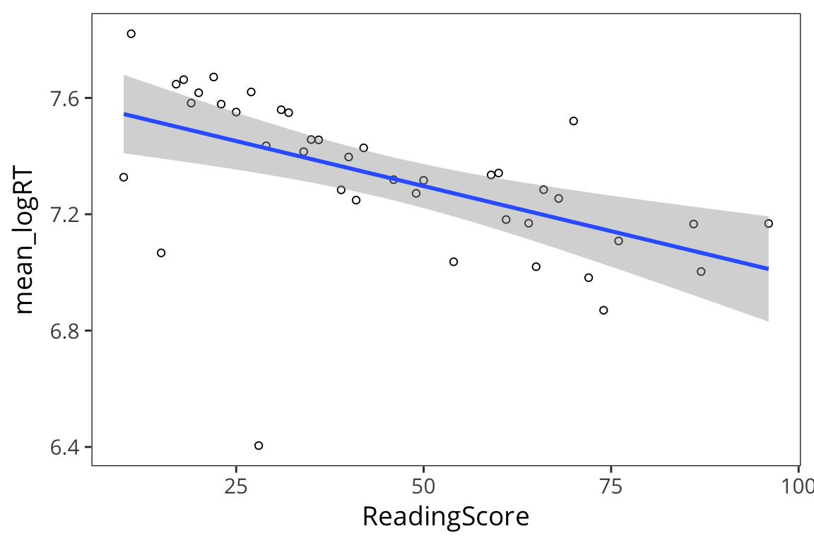
So it looks like there is a relationship between subjects’ reading scores and RTs
all_data %>%
  group_by(LogFamilySize) %>%
  summarise(mean_logRT = mean(LogRT)) %>%
  ggplot(aes(x = LogFamilySize, y = mean_logRT)) +
    geom_point(shape = 1)  +
    geom_smooth(method = "lm")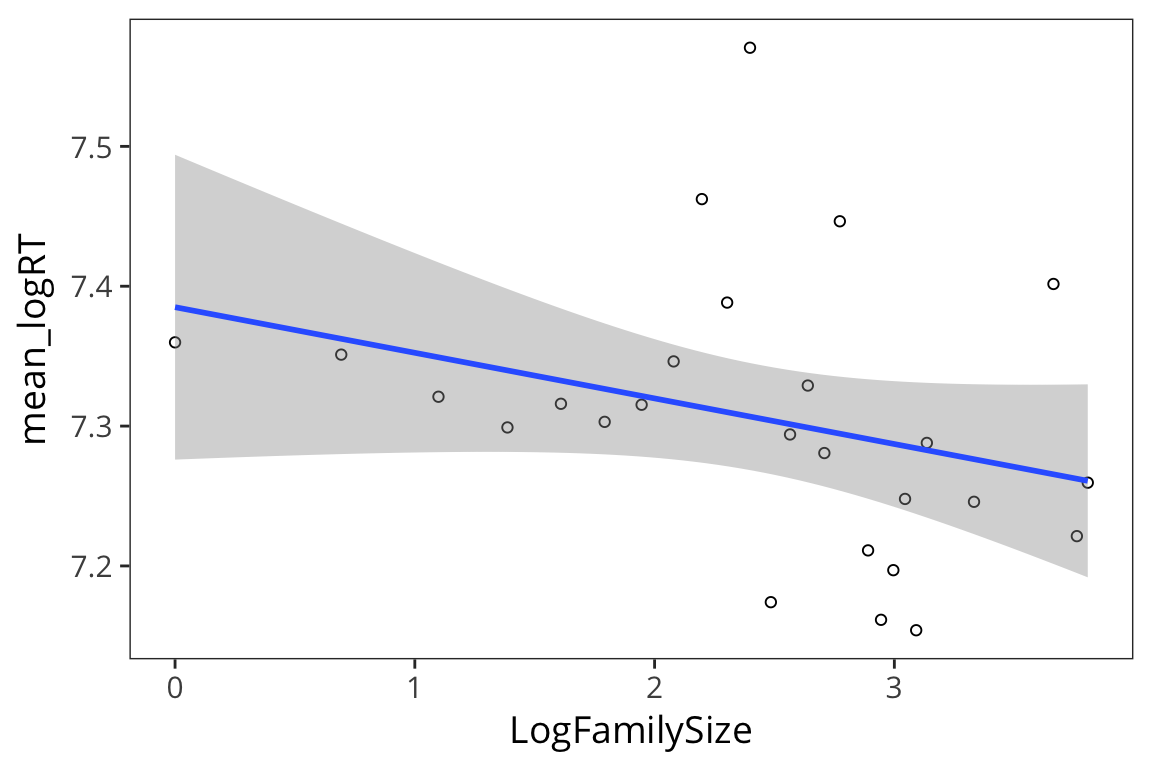
Try it yourself…
- Read in the data we collected in lab on the first day (
in_lab_rts_2018.csv). - Make a new dataset
rt_data_wide, which a) doesn’t contain the “time” column and b) in which there’s one column for each word. HINT: you may want to first unite() 2 columns. Now take
rt_data_wideand make a new dataset,rt_data_long, which has a column for word and a column for trial.rt_data <- read_csv(file.path(data_source, "in_lab_rts_2018.csv")) rt_data_wide <- rt_data %>% select(-time) %>% unite(col = trialinfo, c(trial, word), sep = "_") %>% spread(key = trialinfo, value = rt) rt_data_long <- rt_data_wide %>% gather(key = trialinfo, value = rt, -subject) %>% separate(col = trialinfo, into = c("trial", "word"), sep = "_")
Statistics, continued
Normal distribution review
rts <- read_csv(file.path(data_source, "rts.csv"))

rts <- rts %>%
  mutate(RTlexdec_z = (RTlexdec - mean(RTlexdec)) / sd(RTlexdec)) %>%
  arrange(RTlexdec_z)
If we order all the z-scores from smallest to biggest, what z-score value do we expect 97.5th percentile.
rts$RTlexdec_z[0.975 * nrow(rts)]## [1] 2.089744qnorm(0.975)## [1] 1.959964And conversely we can get the proportion of values below a particular score:
sum(rts$RTlexdec_z < 1.96) / nrow(rts)## [1] 0.9676007pnorm(1.96)## [1] 0.9750021R gives us this function pnorm(), which says the probability that a number drawn from the standard normal distribution is this value or lower.
Try it yourself…
What is the probability that a number drawn from a standard normal is smaller than 3 and larger than -3?
pnorm(3) - pnorm(-3)## [1] 0.9973002Central Limit Theorem
The amazing thing about the normal distribution is how often it comes up. Possibly the most fundamental concept in statistics is the Central Limit Theorem and it explains why we see normal distributions everywhere when we are sampling and summarizing data.
The Central Limit Theorem tells us the following: Given any distribution of some data (including very non-normal distributions), if you take samples of several data points from that distribution and get means of those samples, those means will be normally distributed. This is also true of sds, sums, medians, etc. In addition, the larger the number of data points in your samples, the more the distribution of sample means will be more tightly centered around \(\mu\).
Let’s look at an example to see why this is true.
hist(rts$NounFrequency)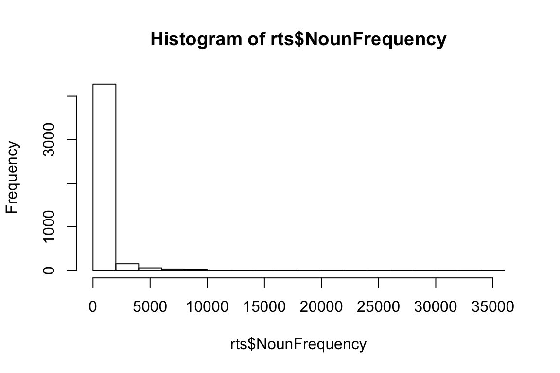
mean(rts$NounFrequency)## [1] 600.1883Let’s draw a bunch of subsamples of the data, and take the mean of each subsample. Then we can look at the distribution over means.
sample_mean <- function(sample_size) {
  resampled_rows <- sample_n(rts, sample_size, replace = TRUE)
  return(mean(resampled_rows$NounFrequency))
}

sample_means <- function(num_samples, sample_size) {
  replicate(num_samples, sample_mean(sample_size))
}
I’m estimating what the distribution of NounFrequency sample means looks like by looking at some number num_samples of samples of size size_of_sample drawn with replacement from my dataset.
Now let’s look at a few different distributions to get a sense of how the estimation is affected by the size of the samples and the amount of resampling.
hist(sample_means(10, 3))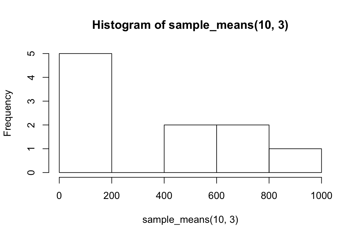
hist(sample_means(100, 3))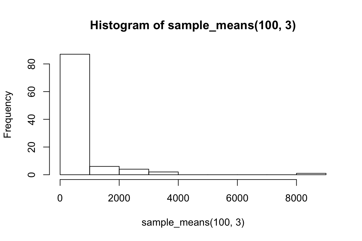
hist(sample_means(1000, 3))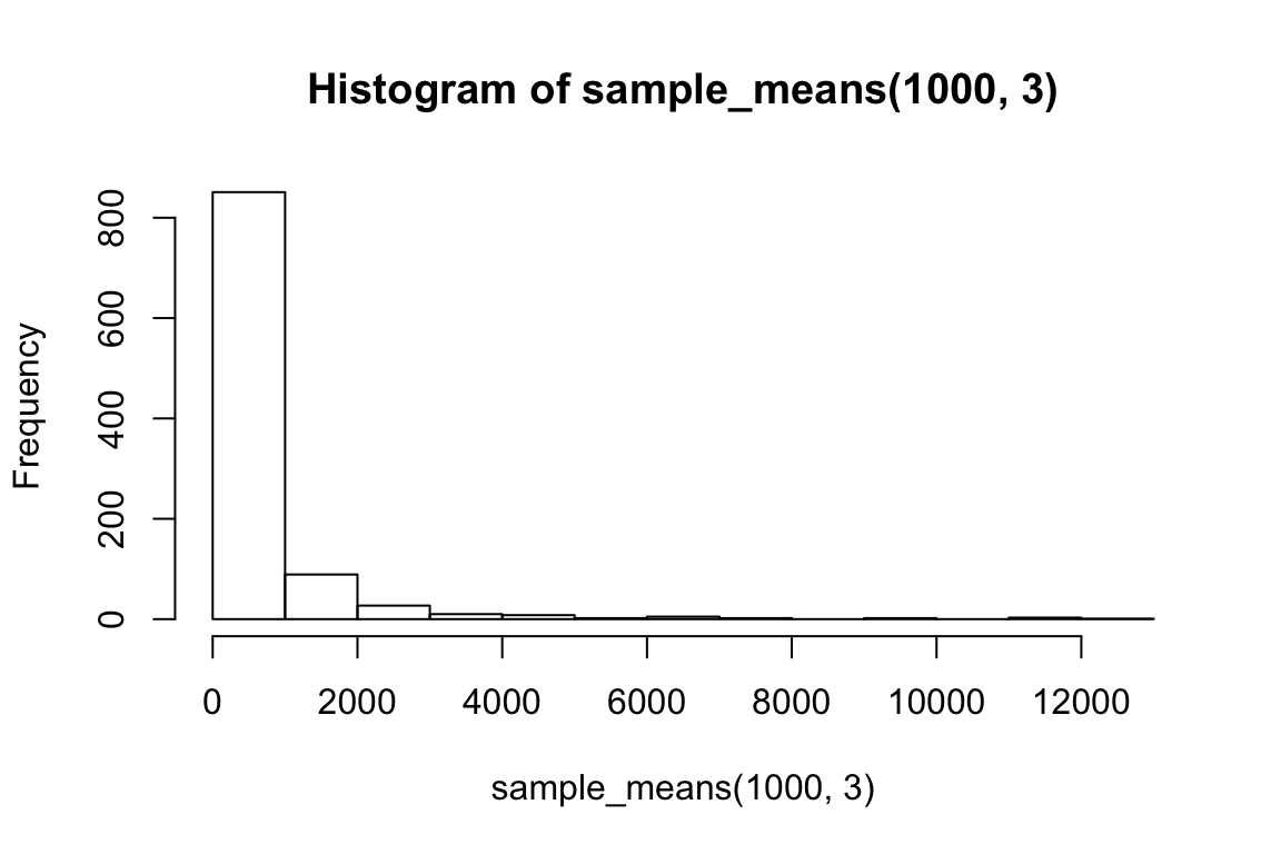
hist(sample_means(100, 100))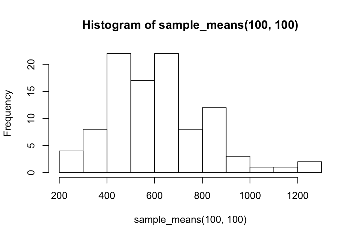
hist(sample_means(1000, 100))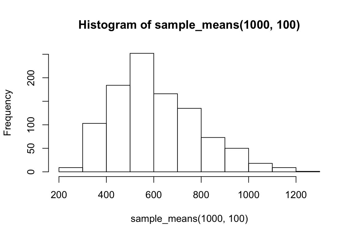
hist(sample_means(1000, 1000))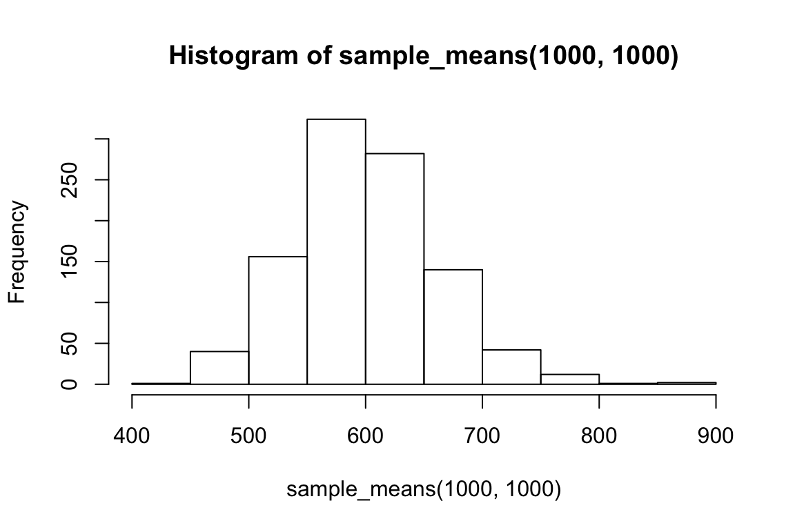
qqnorm(sample_means(1000, 3))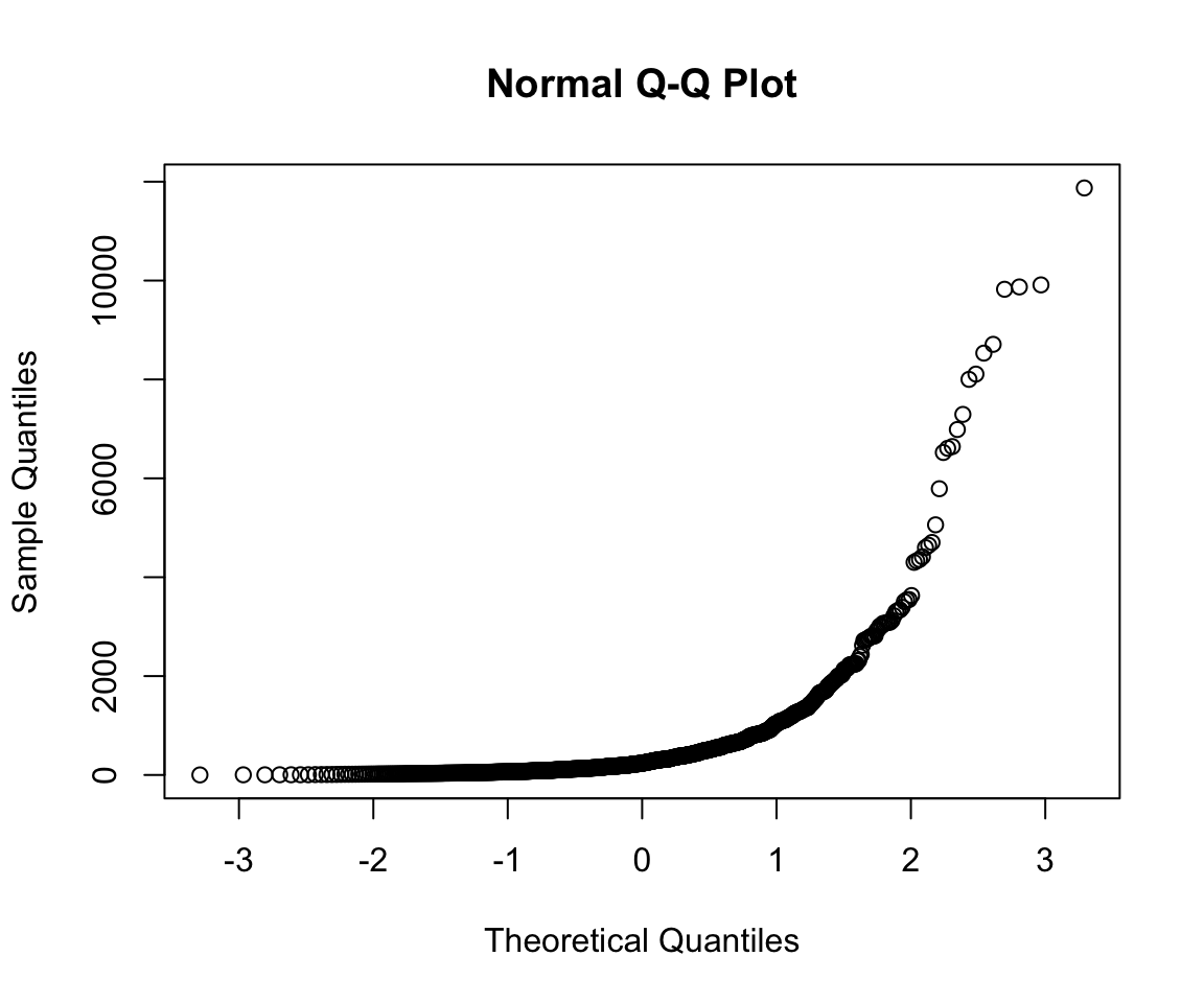
qqnorm(sample_means(100, 1000))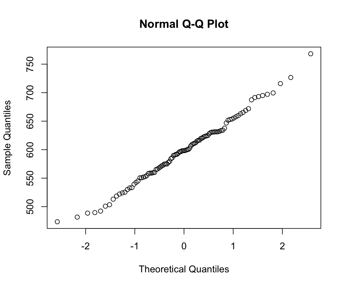
So we can think of data collection during experiments as samples from that underlying distribution. Our goal is to find out its parameters, usually we’re most interested in the location (e.g. mean) but not always. You can see that the size of our sample is going to have an effect on how close we are to the true mean. When we “collected data” from 3 participants we got some pretty out there sample means and so our estimate was way off. But when we “collected” larger samples we were approximating the true mean much more closely.
Try out different distributions and statistics: http://onlinestatbook.com/stat_sim/sampling_dist/.