Lab 6
9.59 Lab in Psycholinguistics
library(tidyverse)
library(broom)
Multiple predictors review
data_source <- "http://web.mit.edu/psycholinglab/data/"
rts <- read_csv(file.path(data_source, "rts.csv"))

ggplot(rts) + geom_histogram(aes(x = RTlexdec), bins = 60, color = "white")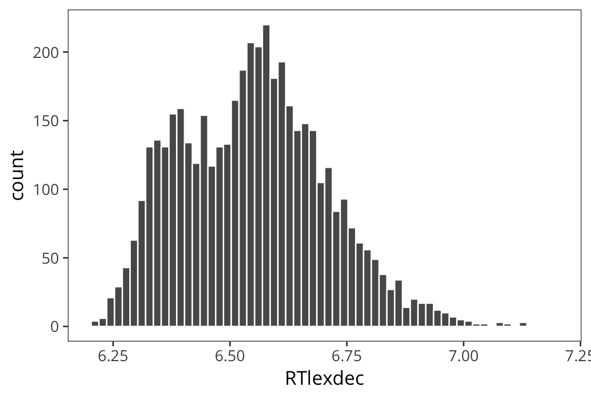
Now remember when we looked at the histogram, we saw that the RTs aren’t quite normally distributed in that there were two peaks. We first tried a linear model with just WrittenFrequency as the predictor.
ggplot(rts, aes(x = WrittenFrequency, y = RTlexdec)) +
  geom_point(aes(colour = AgeSubject), alpha = 0.1) +
  geom_smooth(method = "lm")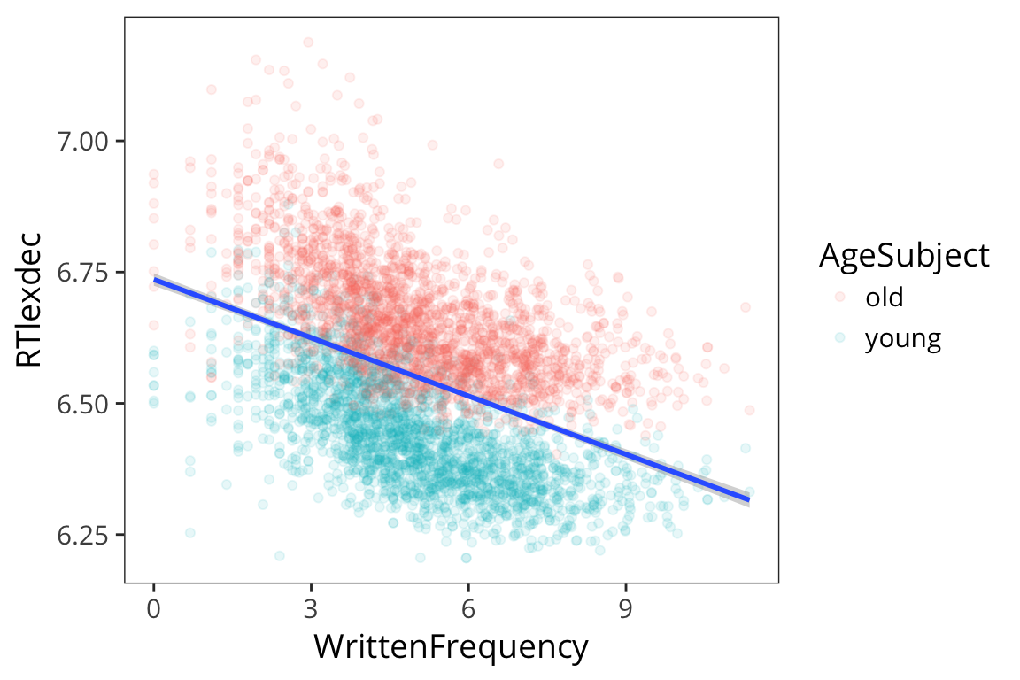
This does an okay job, but we see there are two groups here. Remember we are evaluating our model by seeing how close the fitted values are to the real data points, and we can get a lot closer if we have different lines for different age.
ggplot(rts, aes(x = WrittenFrequency, y = RTlexdec, colour = AgeSubject)) +
  geom_point(alpha = 0.1) +
  geom_smooth(method = "lm")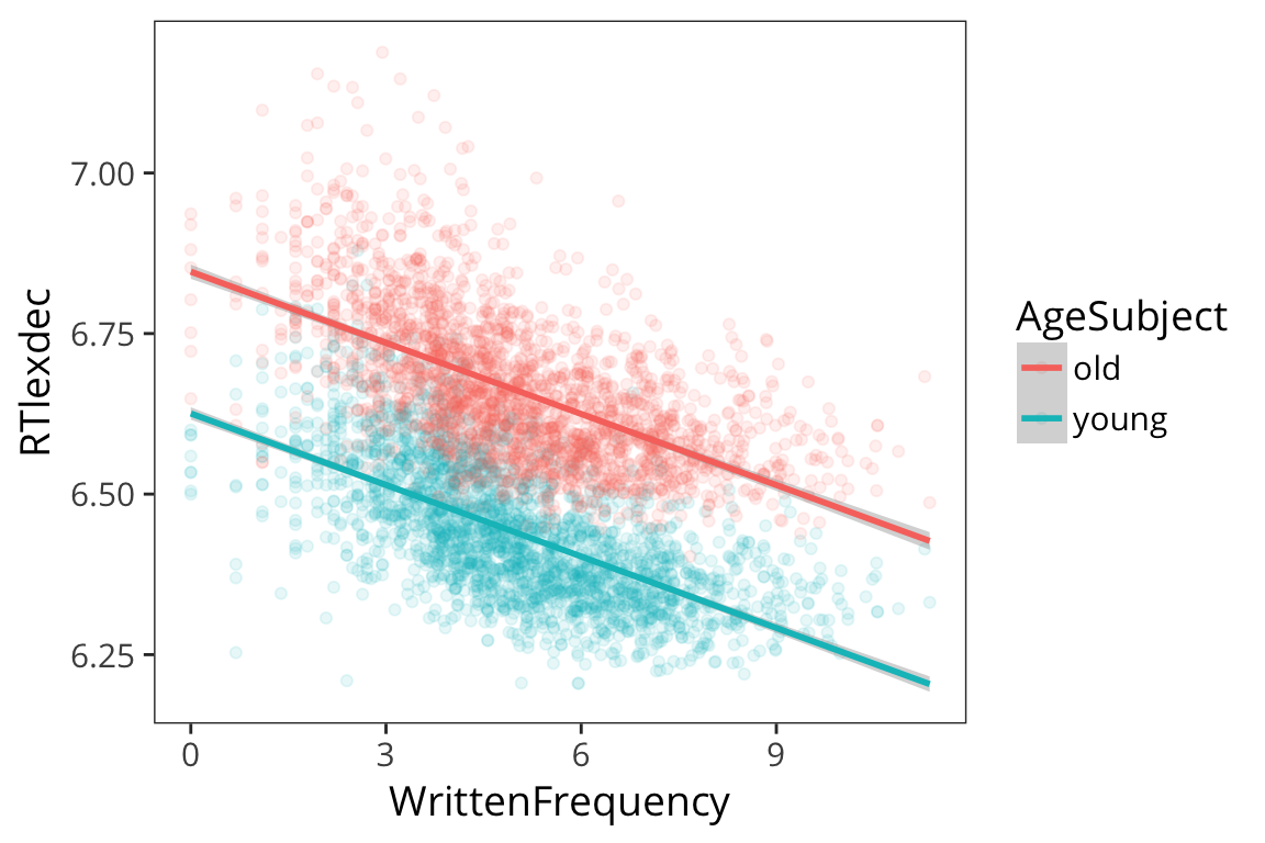
So we ran a regression model with multiple predictors, just adding them together:
rts$AgeSubject <- factor(rts$AgeSubject)
contrasts(rts$AgeSubject) <- c(-0.5, 0.5)

freq_age_lm <- lm(RTlexdec ~ WrittenFrequency + AgeSubject, data = rts)
summary(freq_age_lm)
##
## Call:
## lm(formula = RTlexdec ~ WrittenFrequency + AgeSubject, data = rts)
##
## Residuals:
## Min 1Q Median 3Q Max
## -0.34622 -0.06029 -0.00722 0.05178 0.44999
##
## Coefficients:
## Estimate Std. Error t value Pr(>|t|)
## (Intercept) 6.7359314 0.0037621 1790.48 <2e-16 ***
## WrittenFrequency -0.0370103 0.0007033 -52.62 <2e-16 ***
## AgeSubject1 -0.2217215 0.0025930 -85.51 <2e-16 ***
## ---
## Signif. codes: 0 '***' 0.001 '**' 0.01 '*' 0.05 '.' 0.1 ' ' 1
##
## Residual standard error: 0.08763 on 4565 degrees of freedom
## Multiple R-squared: 0.6883, Adjusted R-squared: 0.6882
## F-statistic: 5040 on 2 and 4565 DF, p-value: < 2.2e-16Try it yourself…
- Recreate the expected values of RTlexdec in each age condition for a WrittenFrequency value of 6 from the estimated parameters above.
Double check your values using
augment().freq_age_results <- tidy(freq_age_lm) intercept <- filter(freq_age_results, term == "(Intercept)")$estimate slope_age <- filter(freq_age_results, term == "AgeSubject1")$estimate slope_freq <- filter(freq_age_results, term == "WrittenFrequency")$estimate old_code <- contrasts(rts$AgeSubject)["old", ] young_code <- contrasts(rts$AgeSubject)["young", ] freq <- 6 # old RTs intercept + freq * slope_freq + old_code * slope_age## old ## 6.62473# young RTs intercept + freq * slope_freq + young_code * slope_age## young ## 6.403009test_data <- data_frame(WrittenFrequency = c(6, 6), AgeSubject = c("old", "young")) augment(freq_age_lm, newdata = test_data)## # A tibble: 2 x 4 ## WrittenFrequency AgeSubject .fitted .se.fit ## <dbl> <chr> <dbl> <dbl> ## 1 6 old 6.624730 0.001958553 ## 2 6 young 6.403009 0.001958553
What do our fitted values look like?
freq_age_aug <- augment(freq_age_lm)

ggplot(freq_age_aug, aes(x = WrittenFrequency, y = RTlexdec,
                         colour = AgeSubject)) +
  geom_point(shape = 1) +
  geom_point(aes(y = .fitted, shape = AgeSubject), colour = "blue", size = 2)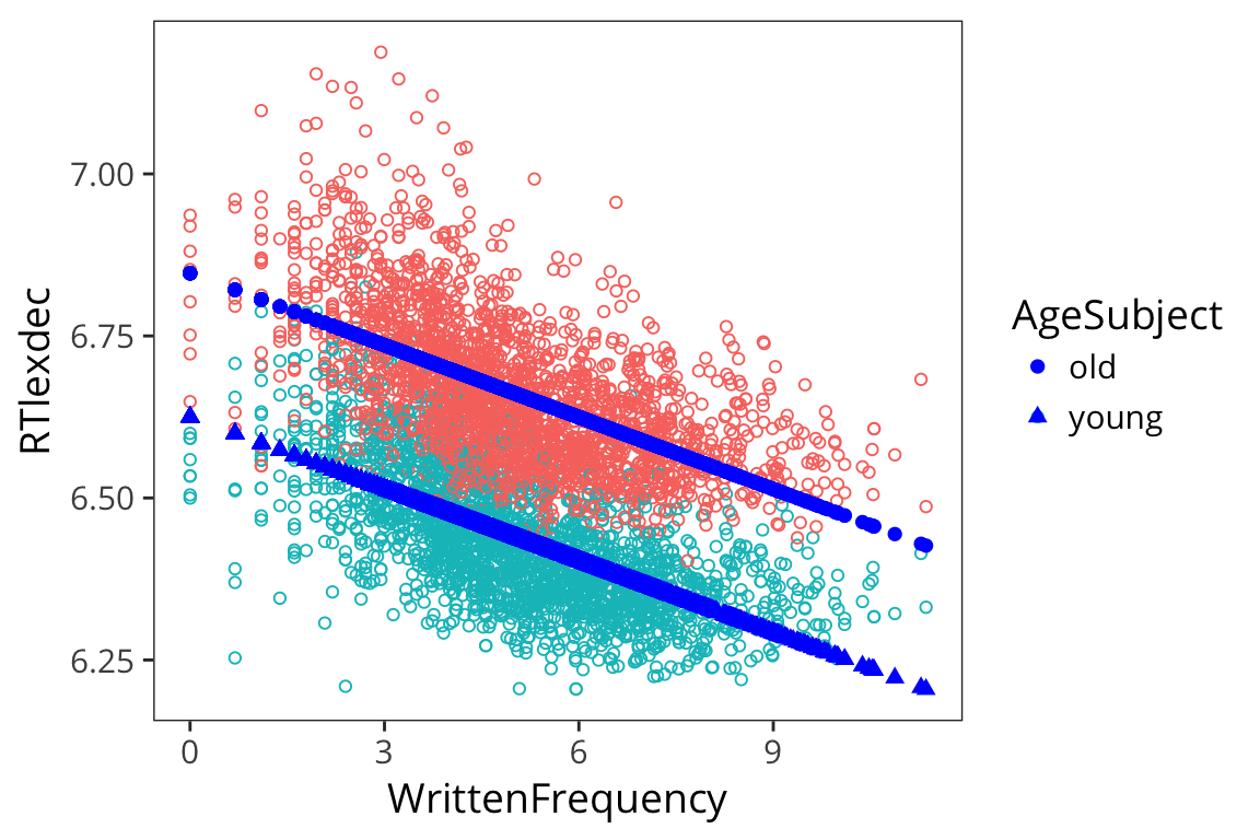
So you can see that you can have multiple continuous predictors, multiple categorical predictors, or a mix of the two in your regression models. This is part of what makes them so useful.
Model comparison
Let’s consider the case of two real-valued predictors. Let’s look at the variable FrequencyInitialDiphoneWord which is the frequency of the first two phonemes in a word. Let’s say you think that frequency is what determines RT, but then someone else thinks initial diphone frequency is what matters. Let’s evaluate that claim.
diphone_lm <- lm(RTlexdec ~ FrequencyInitialDiphoneWord, data = rts)
summary(diphone_lm)
##
## Call:
## lm(formula = RTlexdec ~ FrequencyInitialDiphoneWord, data = rts)
##
## Residuals:
## Min 1Q Median 3Q Max
## -0.35822 -0.12515 -0.00013 0.10336 0.63291
##
## Coefficients:
## Estimate Std. Error t value Pr(>|t|)
## (Intercept) 6.593868 0.015354 429.470 < 2e-16 ***
## FrequencyInitialDiphoneWord -0.004225 0.001465 -2.884 0.00395 **
## ---
## Signif. codes: 0 '***' 0.001 '**' 0.01 '*' 0.05 '.' 0.1 ' ' 1
##
## Residual standard error: 0.1568 on 4566 degrees of freedom
## Multiple R-squared: 0.001818, Adjusted R-squared: 0.0016
## F-statistic: 8.317 on 1 and 4566 DF, p-value: 0.003945We see that initial diphone frequency does predict RT. But what if we include both predictors, initial diphone frequency and written frequency?
freq_diphone_lm <- lm(RTlexdec ~ WrittenFrequency + FrequencyInitialDiphoneWord, data = rts)
summary(freq_diphone_lm)
##
## Call:
## lm(formula = RTlexdec ~ WrittenFrequency + FrequencyInitialDiphoneWord,
## data = rts)
##
## Residuals:
## Min 1Q Median 3Q Max
## -0.45641 -0.11701 -0.00141 0.10359 0.56127
##
## Coefficients:
## Estimate Std. Error t value Pr(>|t|)
## (Intercept) 6.7315271 0.0144749 465.047 <2e-16 ***
## WrittenFrequency -0.0370517 0.0011412 -32.468 <2e-16 ***
## FrequencyInitialDiphoneWord 0.0004452 0.0013285 0.335 0.738
## ---
## Signif. codes: 0 '***' 0.001 '**' 0.01 '*' 0.05 '.' 0.1 ' ' 1
##
## Residual standard error: 0.1413 on 4565 degrees of freedom
## Multiple R-squared: 0.1891, Adjusted R-squared: 0.1887
## F-statistic: 532.2 on 2 and 4565 DF, p-value: < 2.2e-16What does this mean? When you have two linear predictors, and try to find coefficients that minimize the squared distance to datapoints, then to get the best coefficients, you try to estimate what is the effect of variable a while holding variable b constant, and what is the effect of variable b while holding variable a constant. So this means, approximately, whole holding WrittenFrequency constant, initial diphone has this effect on RTs, which is not significant. And controlling for initial diphone frequency – holding it constant – we estimate this is the slope for WrittenFrequency, basically the same slope as we found before.
This offers some evidence that WrittenFrequency is what matters here, not initial diphone frequency. You often find yourself in the position where there are multiple things that predict patterns in your dataset, and you want to figure out which one is more basic, or which one causes the others, or which one is real and which one is confounded.
This kind of test offers some evidence about that question, but there are lots and lots of caveats to interpreting this p-value this way. There are better tests to do. The principle thing that makes this hard to interpret is that the controlling is mutual here: this is the effect of written frequency after holding initial diphone frequency constant, and vice versa.
Basically, you can trust this kind of test for two variables that are not highly correlated.
These two variables aren’t highly correlated, so this kind of hypothesis testing makes sense.
cor(rts$WrittenFrequency, rts$FrequencyInitialDiphoneWord)## [1] 0.108279Interactions
So far in all these models we’ve entered multiple predictors that can exert their effects somewhat independently, but what if things are more complicated and they actually interact?
For example, what if for young people, more frequent words had faster RTs, but for old people, it was the opposite?
This isn’t the case in our data but let’s make it the case for illusrtration purposes.
rts_mod <- rts %>%
  mutate(RTfake = if_else(AgeSubject == "old", 14 - RTlexdec, RTlexdec))

ggplot(rts_mod, aes(x = WrittenFrequency, y = RTfake)) +
  geom_point(aes(colour = AgeSubject), alpha = 0.2) +
  geom_smooth(method = "lm")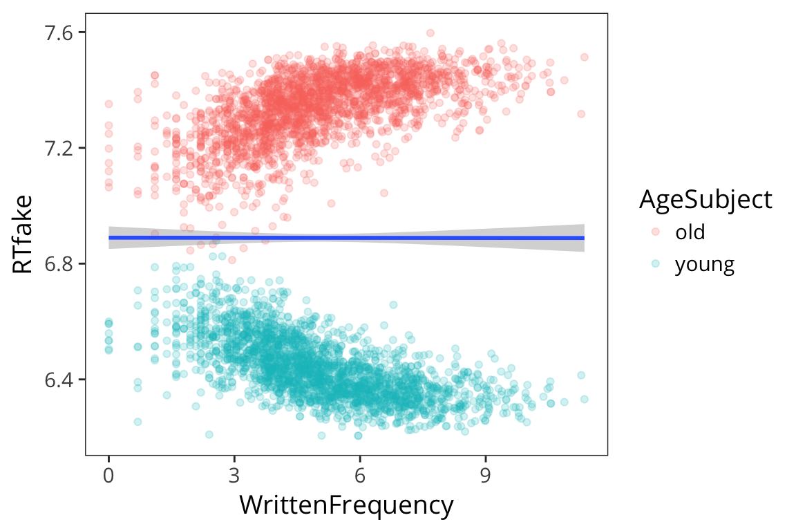
If we analyze this the way we did before:
mod_lm <- lm(RTfake ~ WrittenFrequency + AgeSubject, data = rts_mod)
summary(mod_lm)
##
## Call:
## lm(formula = RTfake ~ WrittenFrequency + AgeSubject, data = rts_mod)
##
## Residuals:
## Min 1Q Median 3Q Max
## -0.52705 -0.07503 0.00187 0.08003 0.43968
##
## Coefficients:
## Estimate Std. Error t value Pr(>|t|)
## (Intercept) 6.890e+00 4.768e-03 1444.846 <2e-16 ***
## WrittenFrequency -9.664e-05 8.915e-04 -0.108 0.914
## AgeSubject1 -8.998e-01 3.287e-03 -273.774 <2e-16 ***
## ---
## Signif. codes: 0 '***' 0.001 '**' 0.01 '*' 0.05 '.' 0.1 ' ' 1
##
## Residual standard error: 0.1111 on 4565 degrees of freedom
## Multiple R-squared: 0.9426, Adjusted R-squared: 0.9426
## F-statistic: 3.748e+04 on 2 and 4565 DF, p-value: < 2.2e-16We see no effect of WrittenFrequency which is clearly wrong it’s just that it’s getting obscured by the fact that it’s in opposite directions for each age group.
So how can we include the fact that the effect of writtenFrequency varies depending on which value of AgeSubject:
\[ \text{RTlexdec} = \beta_0 + \beta_1 \cdot \text{WrittenFreqeuncy} + \beta_2 \cdot \text{AgeSubject} + \beta_3 \cdot \text{WrittenFreqeuncy} \cdot \text{AgeSubject} + \mathcal{N}(0, \sigma) \]
This multiplicative term is called an interaction.
mod_int_lm <- lm(RTfake ~ WrittenFrequency * AgeSubject, data = rts_mod)
summary(mod_int_lm)
##
## Call:
## lm(formula = RTfake ~ WrittenFrequency * AgeSubject, data = rts_mod)
##
## Residuals:
## Min 1Q Median 3Q Max
## -0.45019 -0.05438 0.00128 0.05936 0.34877
##
## Coefficients:
## Estimate Std. Error t value Pr(>|t|)
## (Intercept) 6.890e+00 3.762e-03 1831.138 <2e-16 ***
## WrittenFrequency -9.664e-05 7.034e-04 -0.137 0.891
## AgeSubject1 -5.281e-01 7.525e-03 -70.185 <2e-16 ***
## WrittenFrequency:AgeSubject1 -7.402e-02 1.407e-03 -52.615 <2e-16 ***
## ---
## Signif. codes: 0 '***' 0.001 '**' 0.01 '*' 0.05 '.' 0.1 ' ' 1
##
## Residual standard error: 0.08764 on 4564 degrees of freedom
## Multiple R-squared: 0.9643, Adjusted R-squared: 0.9642
## F-statistic: 4.105e+04 on 3 and 4564 DF, p-value: < 2.2e-16So what this is saying is that there is no main effect of WrittenFrequency but there is a main effect of AgeSubject (younger people are faster) and the interaction between AgeSubject and WrittenFrequency is significant. The significance of the interaction term here means that the slope on top is significantly different from the slope on the bottom.
A note about the coding:
So if we go back to the dummy coding and rerun the model…
contrasts(rts_mod$AgeSubject)## [,1]
## old -0.5
## young 0.5contrasts(rts_mod$AgeSubject) <- c(0, 1)
contrasts(rts_mod$AgeSubject)## [,1]
## old 0
## young 1mod_int_lm_2 <- lm(RTfake ~ WrittenFrequency * AgeSubject, data = rts_mod)
summary(mod_int_lm_2)##
## Call:
## lm(formula = RTfake ~ WrittenFrequency * AgeSubject, data = rts_mod)
##
## Residuals:
## Min 1Q Median 3Q Max
## -0.45019 -0.05438 0.00128 0.05936 0.34877
##
## Coefficients:
## Estimate Std. Error t value Pr(>|t|)
## (Intercept) 7.1536932 0.0053210 1344.44 <2e-16 ***
## WrittenFrequency 0.0369136 0.0009948 37.11 <2e-16 ***
## AgeSubject1 -0.5281373 0.0075250 -70.19 <2e-16 ***
## WrittenFrequency:AgeSubject1 -0.0740206 0.0014068 -52.62 <2e-16 ***
## ---
## Signif. codes: 0 '***' 0.001 '**' 0.01 '*' 0.05 '.' 0.1 ' ' 1
##
## Residual standard error: 0.08764 on 4564 degrees of freedom
## Multiple R-squared: 0.9643, Adjusted R-squared: 0.9642
## F-statistic: 4.105e+04 on 3 and 4564 DF, p-value: < 2.2e-16What you’re getting here is a significant effect of WrittenFrequency because it’s looking only at the effect of WrittenFrequency for AgeSubject = 0 (i.e. old) –> this is a simple effect.
When we had the effects coding, WrittenFrequency was being measured across both levels Age so there was no main effect of WrittenFreqeuncy. Everything else about the model looks about the same, but if you don’t know what coding scheme you used, you can’t interpret the effects. People misunderstand this ALL THE TIME.
Logistic regression
So far we’ve dealt with data where the dependent variable is some continuous quantity, in this case we’ve looked at RTs. But often in linguistics we want to answer a categorical question. For example, we may want to see what predicts people’s tendency to say “yes” or “no”, as in the typical comprehension question. In cases where the possible values of the dependent variable are 0 or 1, it’s no longer appropriate to use linear regression, because linear regression produces values all over the number line.
For this part, let’s imagine that we care about slow vs. fast RTs more coarsely.
rts_binary <- rts %>%
  mutate(rt_binary = if_else(RTlexdec > 6.5, 1, 0))

ggplot(rts_binary, aes(x = WrittenFrequency, y = rt_binary)) +
  geom_point(shape = 1) +
  geom_smooth(method = "glm", method.args = list(family = "binomial"))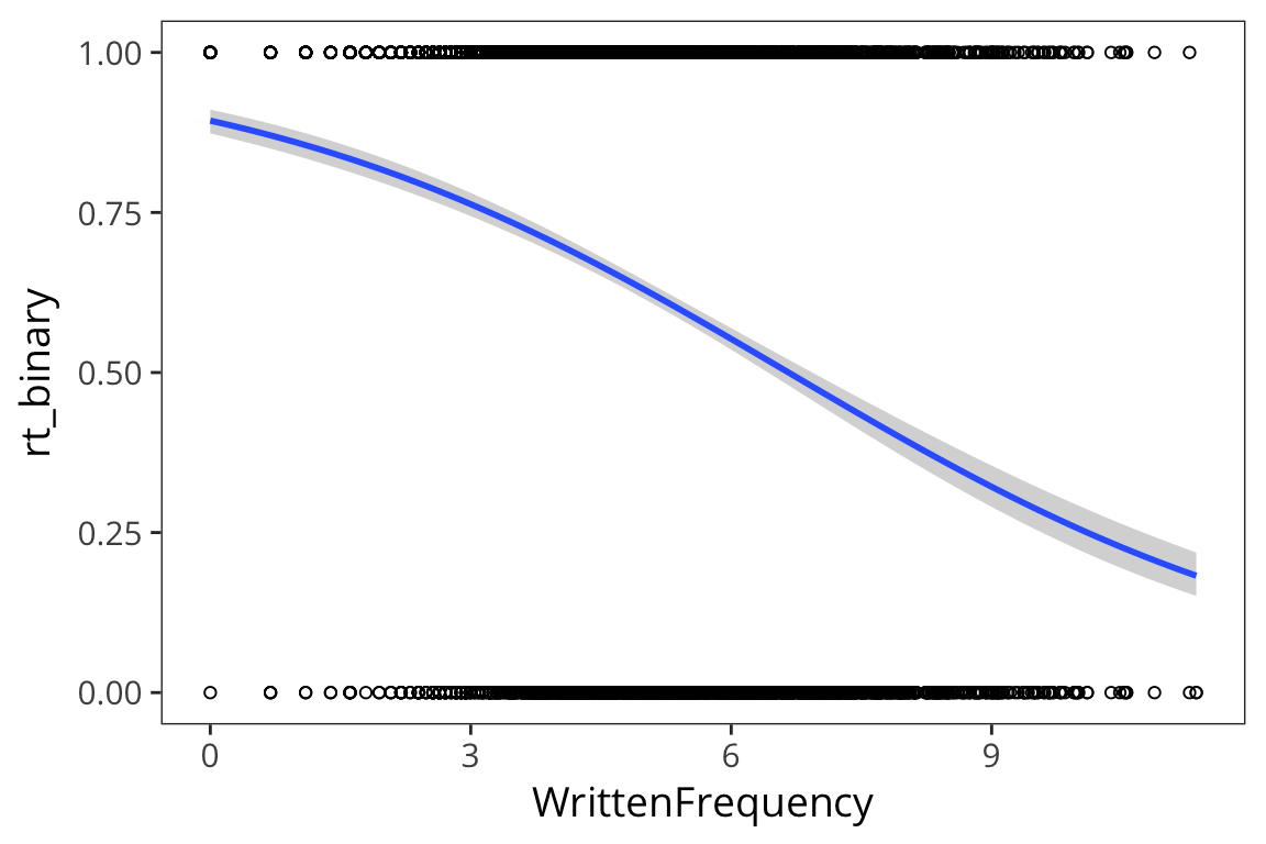
You can see that all the values are 0s and 1s so that makes it hard to see a pattern
Let’s bin the x-axis and get means within each bin just to get an idea…
rts_binned <- rts_binary %>%
  mutate(freq_bin = cut(WrittenFrequency, 20)) %>%
  group_by(freq_bin) %>%
  summarise(mean_rt = mean(rt_binary))

ggplot(rts_binned, aes(x = freq_bin, y = mean_rt)) +
  geom_point() +
  theme(axis.text.x = element_text(angle = 45, hjust = 1, size = 8))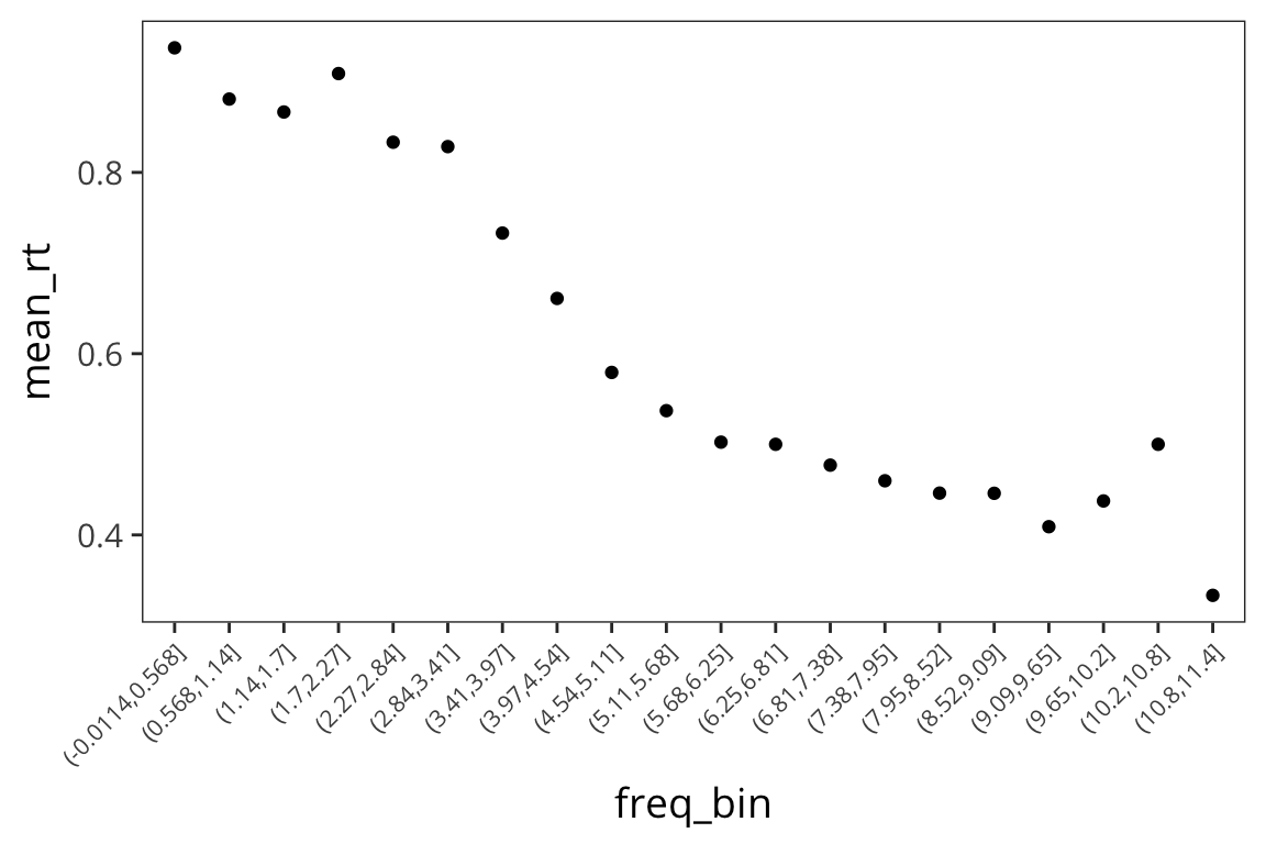
So we see a familiar relationship: the higher the written frequency, the more likely that the average RT is closer to 0.
But rt_binary is a binary variable (1 or 0) so if we want that to be our outcome, the normal distribution is not appropriate. The errors are not normally distributed around the expected values – it’s all 0s and 1s. We’re no longer interested in predicting number values, but rather in classifying our data as 0 or 1. Our generative process should be something that gets a probability that something is in class 1, then flips a coin with that probability to determine its class.
Instead of a normal distribution here, let’s use a bernoulli distribution. A bernoulli distribution takes one parameter, called \(p\), and returns 1 with probability \(p\), and 0 with probability \(1 - p\).
rbernoulli(n = 10, p = 0.5)## [1] TRUE FALSE FALSE FALSE FALSE FALSE TRUE FALSE FALSE TRUESo we can still use the concepts from linear regression where we have an intercept \(\beta_0\) and slope \(\beta_1\) to figure out the probability of a \(y\) being 1 or 0 given a certain \(x\) and then submit that to the bernoulli distribution.
\[ p = \beta_0 + \beta_1 \cdot x_1 + \beta_2 \cdot x_2 + ... \] \[ y \sim \text{Bernoulli}(p) \]
Okay, but the problem is a probability has to be between 0 and 1, and there’s no guarantee that this expression will do that. In our expression so far, p could be any real number from negative infinity to infinity. So let’s just run it through a function which takes real numbers, then squashes them into the space between 0 and 1 by generating values that are like .9999 or .97 or .0001. So we want the values coming out of our model to be really close to 1, or really close to 0, which is similar to our real data. Then if the value is less than .5 we count that as a prediction of 0 and if it’s greater than .5 we count it as a prediction of 1.
That is the logistic function. In particular it makes 0 into .5.
logistic <- function(x) {
  exp(x) / (1 + exp(x))
}

xs <- runif(10000, -10, 10)
qplot(xs, logistic(xs))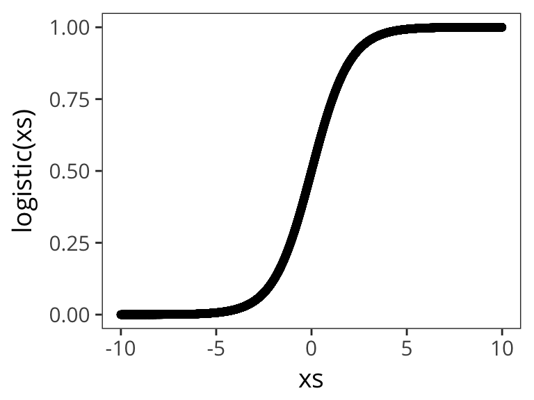
Let’s try out a few different possible \(\beta_0\) and \(\beta_1\) values to get a sense of how the logistic function changes as function of them:
qplot(xs, logistic( 1 + 0.5 * xs))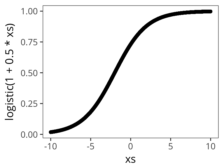
qplot(xs, logistic( 3 + 0.5 * xs))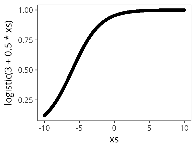
qplot(xs, logistic( 3 + 3 * xs))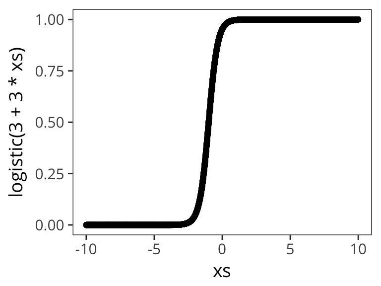
qplot(xs, logistic( 1 + 3 * xs))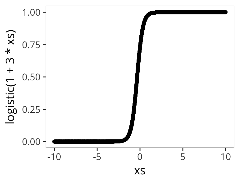
qplot(xs, logistic( 3 - 0.5 * xs))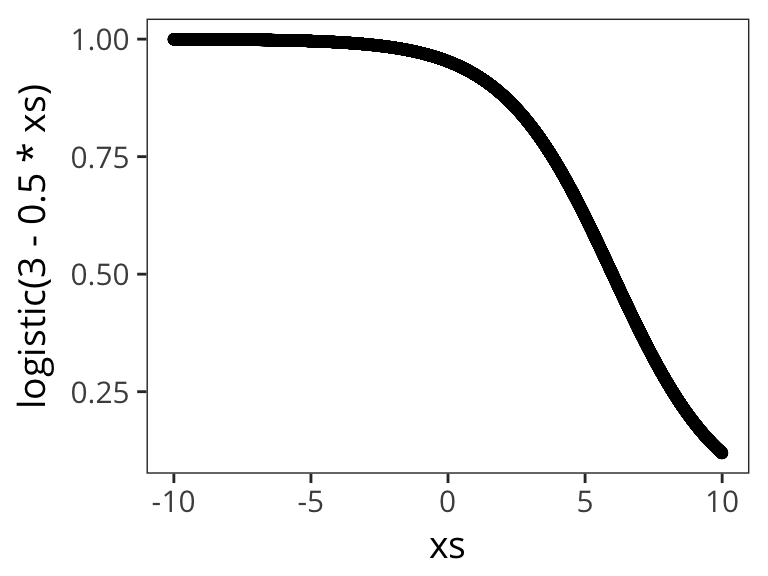
qplot(xs, logistic( 0.1 - 0.5 * xs))
qplot(xs, logistic( 0.1 - 5 * xs))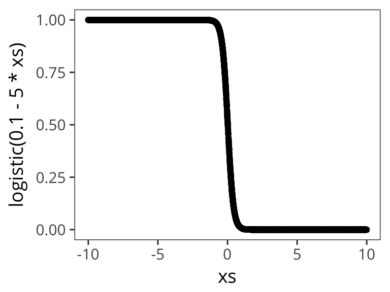
qplot(xs, logistic(-1 - 0.5 * xs))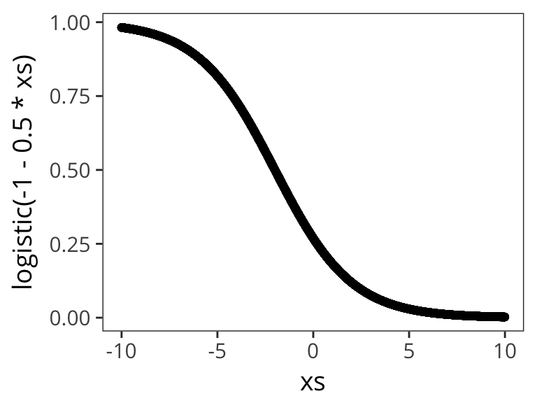
Now we’ll say:
\[ p = \text{logistic}( \beta_0 + \beta_1 \cdot x_1 + \beta_2 \cdot x_2 + ... ) \]
So let’s run a logistic regression. The syntax is very similar to linear regression:
freq_glm <- glm(rt_binary ~ WrittenFrequency, data = rts_binary,
                family = binomial(link = "logit"))
summary(freq_glm)
##
## Call:
## glm(formula = rt_binary ~ WrittenFrequency, family = binomial(link = "logit"),
## data = rts_binary)
##
## Deviance Residuals:
## Min 1Q Median 3Q Max
## -2.1163 -1.2300 0.7402 0.9421 1.8335
##
## Coefficients:
## Estimate Std. Error z value Pr(>|z|)
## (Intercept) 2.12664 0.09975 21.32 <2e-16 ***
## WrittenFrequency -0.31928 0.01813 -17.61 <2e-16 ***
## ---
## Signif. codes: 0 '***' 0.001 '**' 0.01 '*' 0.05 '.' 0.1 ' ' 1
##
## (Dispersion parameter for binomial family taken to be 1)
##
## Null deviance: 6068.0 on 4567 degrees of freedom
## Residual deviance: 5726.2 on 4566 degrees of freedom
## AIC: 5730.2
##
## Number of Fisher Scoring iterations: 4freq_glm_tidy <- tidy(freq_glm)
intercept <- filter(freq_glm_tidy, term == "(Intercept)")$estimate
slope <- filter(freq_glm_tidy, term == "WrittenFrequency")$estimate
newxs <- runif(10000, 0, 10)
freq_logistic <- logistic(intercept + slope * newxs)
qplot(newxs, freq_logistic)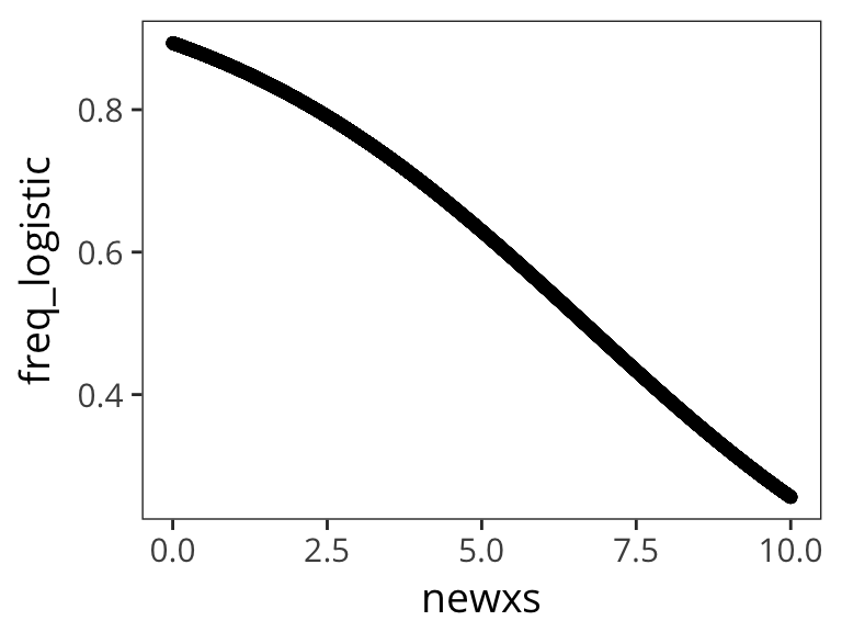
At the top we have some information about the residuals (same as with linear regression), but here they don’t need to be normally distributed.
At the very bottom there are some descriptions of how well the model is fitting the data. One test asks whether the model with predictors fits significantly better than a model with just an intercept (i.e., a null model). The test statistic is the difference between the residual deviance for the model with predictors and the null model. It is chi-square distributed with degrees of freedom equal to the differences in degrees of freedom between the current and the null model (i.e. the number of predictor variables in the model). You could compute it but it’s not super informative. AIC is similar - it’s useful for comparing models. The iteration is a measure of how much time it took to find the best estimate.
Now the coefficients are somewhat harder to interpret than in linear regression:
The intercept corresponds to the log odds of being in the slow RT group (RTbin=1) when WrittenFrequency is 0. In other words, the odds of being slow for words with frequency 0 is pretty high. In this case this is not super useful information. In general, the intercept is often less interesting in logistic regression.
Earlier, we could say that the slope corresponded the change in \(y\) for 1 unit change of \(x\). Here, it’s the same thing, but then squashed in the logistic function, so it’s a little harder to map onto some meaningful numbers.
Let’s see what happens if we pull out some plausible values of frequency.
# probability of slow given frequency = 5
logistic(intercept + slope * 5)
## [1] 0.6295346# probability of slow given frequency = 6
logistic(intercept + slope * 6)## [1] 0.5525395predicted <- augment(freq_glm, newdata = data_frame(WrittenFrequency = c(5, 6)),
type.predict = "response")So the log odds of a slow RT, when Frequency is 5, are 0.63 and the log odds of a slow RT are 0.55 for Frequency = 6. Now we can reconstruct the slope by looking at a 1 unit increase in Frequency by taking the difference of the log odds.
log_odds_5 <- log(predicted$.fitted[1] / (1 - predicted$.fitted[1]))
log_odds_6 <- log(predicted$.fitted[2] / (1 - predicted$.fitted[2]))

diff_log_odds <- log_odds_6 - log_odds_5
diff_log_odds
## [1] -0.3192841You can still take a larger slope to indicate a larger effect, but now instead of 1 unit change in \(x\) being equal to 1 unit change in \(y\), it means 1 unit change in WrittenFrequency corresponds to a -0.32 change in log odds of RTbin being 1, i.e. of a slow reaction time.
It’s pretty hard to imagine what it means for something to decrease in log-odds space. By exponentiating we can think about the odds ratio (odds for \(x=6\) / odds for \(x=5\)).
exp(diff_log_odds)## [1] 0.7266691This says that the odds of RT being categorized as slow are multiplied by 0.73 (i.e. < 1 means decreases) with every additional unit of WrittenFrquency.
Because the relationship between \(p(x)\) and \(x\) is not linear, we can’t easily say anything about the change in proportions for a unit change in \(x\).
What about categorical predictors?
You can use the same dummy coding or deviation coding approach as before:
contrasts(rts_binary$AgeSubject) ## [,1]
## old -0.5
## young 0.5age_glm <- glm(rt_binary ~ AgeSubject, data = rts_binary,
family = binomial(link = "logit"))
summary(age_glm)##
## Call:
## glm(formula = rt_binary ~ AgeSubject, family = binomial(link = "logit"),
## data = rts_binary)
##
## Deviance Residuals:
## Min 1Q Median 3Q Max
## -2.6242 -0.7959 0.2549 0.2549 1.6149
##
## Coefficients:
## Estimate Std. Error z value Pr(>|z|)
## (Intercept) 1.21174 0.06396 18.95 <2e-16 ***
## AgeSubject1 -4.39800 0.12792 -34.38 <2e-16 ***
## ---
## Signif. codes: 0 '***' 0.001 '**' 0.01 '*' 0.05 '.' 0.1 ' ' 1
##
## (Dispersion parameter for binomial family taken to be 1)
##
## Null deviance: 6068.0 on 4567 degrees of freedom
## Residual deviance: 3317.3 on 4566 degrees of freedom
## AIC: 3321.3
##
## Number of Fisher Scoring iterations: 6age_glm_tidy <- tidy(age_glm)
intercept <- filter(age_glm_tidy, term == "(Intercept)")$estimate
slope <- filter(age_glm_tidy, term == "AgeSubject1")$estimate
old_code <- contrasts(rts_binary$AgeSubject)["old", ]
young_code <- contrasts(rts_binary$AgeSubject)["young", ]
# probability of slow given old
logistic(intercept + slope * old_code)## old
## 0.9680385# probability of slow given young
logistic(intercept + slope * young_code)## young
## 0.2714536ggplot(rts_binary, aes(x = WrittenFrequency, y = rt_binary, colour = AgeSubject)) +
geom_point(shape = 1) +
geom_smooth(method = "glm", method.args = list(family = "binomial"))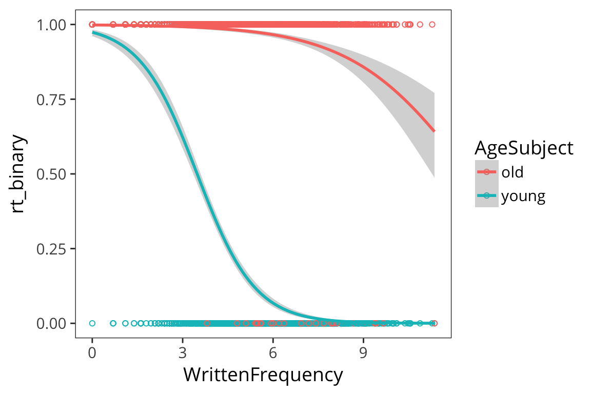
freq_age_glm <- glm(rt_binary ~ AgeSubject * WrittenFrequency, data = rts_binary,
                    family = binomial(link = "logit"))
summary(freq_age_glm)
##
## Call:
## glm(formula = rt_binary ~ AgeSubject * WrittenFrequency, family = binomial(link = "logit"),
## data = rts_binary)
##
## Deviance Residuals:
## Min 1Q Median 3Q Max
## -2.9953 -0.3450 0.1479 0.2803 3.1620
##
## Coefficients:
## Estimate Std. Error z value Pr(>|z|)
## (Intercept) 5.03088 0.24681 20.384 < 2e-16 ***
## AgeSubject1 -2.81379 0.49361 -5.700 1.20e-08 ***
## WrittenFrequency -0.77854 0.04065 -19.150 < 2e-16 ***
## AgeSubject1:WrittenFrequency -0.52569 0.08131 -6.465 1.01e-10 ***
## ---
## Signif. codes: 0 '***' 0.001 '**' 0.01 '*' 0.05 '.' 0.1 ' ' 1
##
## (Dispersion parameter for binomial family taken to be 1)
##
## Null deviance: 6068.0 on 4567 degrees of freedom
## Residual deviance: 2462.2 on 4564 degrees of freedom
## AIC: 2470.2
##
## Number of Fisher Scoring iterations: 7Linear mixed-effects models
One important assumption of all these models is that we have been pretending that all the data points in our scatter plot are generated independently from calls to some generative process like rnorm. But that’s not how experiments usually work…
Usually each subject sees a bunch of items in one of several conditions. And the same items are seen by many subjects (sometimes there are different lists but sometimes all subjects see all items).
There will be some correlation between datapoints within subjects, because maybe some subjects are sleepy and tend to respond slowly, or others just drank a bunch of coffee and are responding super fast. This correlation is entirely missed in our regression model here. We’re analyzing our data as if it was between-subjects, and consequently we’re losing statistical power. Same thing with the items. We know now that words have properties that affect how people respond to them so subjects’ responses will be correlated for a the same items.
Let’s look at this in the lexdec dataset:
library(languageR)

ggplot(lexdec, aes(x = Trial, y = RT)) +
  geom_point(shape = 1)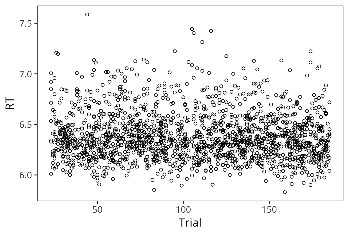
lexdec_subject <- lexdec %>%
  group_by(Subject) %>%
  summarise(mean_rt = mean(RT))

ggplot(lexdec, aes(x = Subject, y = RT)) +
  geom_point(shape = 1, colour = "grey") +
  geom_point(aes(y = mean_rt), data = lexdec_subject, size = 3)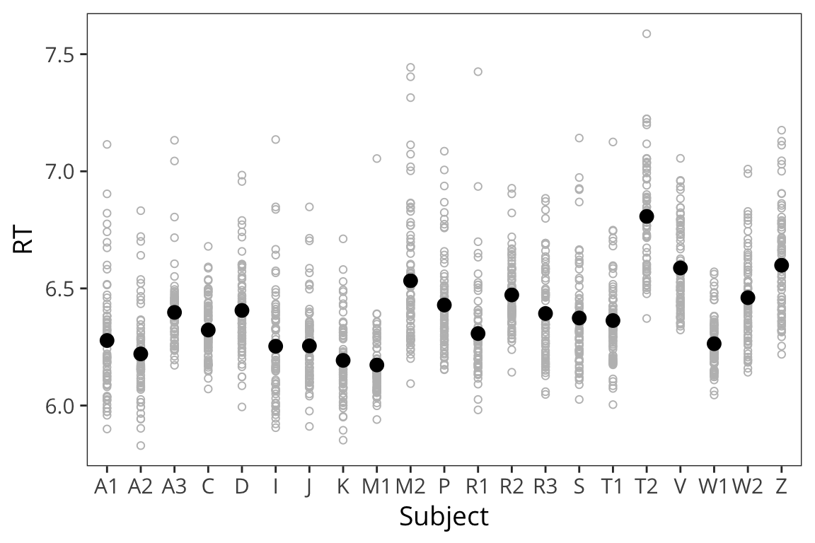
You can see that the different subjects have different average RTs and they also vary in terms of how they are affected by the the predictor of interest:
ggplot(lexdec, aes(x = Trial, y = RT)) +
  facet_wrap(~Subject) +
  geom_point(shape = 1) +
  geom_smooth(method = "lm")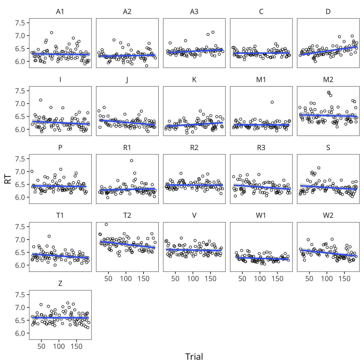
Same thing if we look at items:
lexdec_items <- lexdec %>%
  group_by(Word) %>%
  summarise(mean_rt = mean(RT))

ggplot(lexdec_items, aes(x = Word, y = mean_rt)) +
  geom_text(aes(label = Word)) +
  theme(axis.text.x = element_text(angle = 45, hjust = 1, size = 8))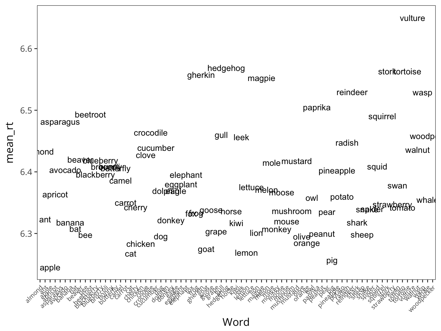
ggplot(lexdec, aes(x = Trial, y = RT)) +
  facet_wrap(~Word) +
  geom_point(shape = 1) +
  geom_smooth(method = "lm")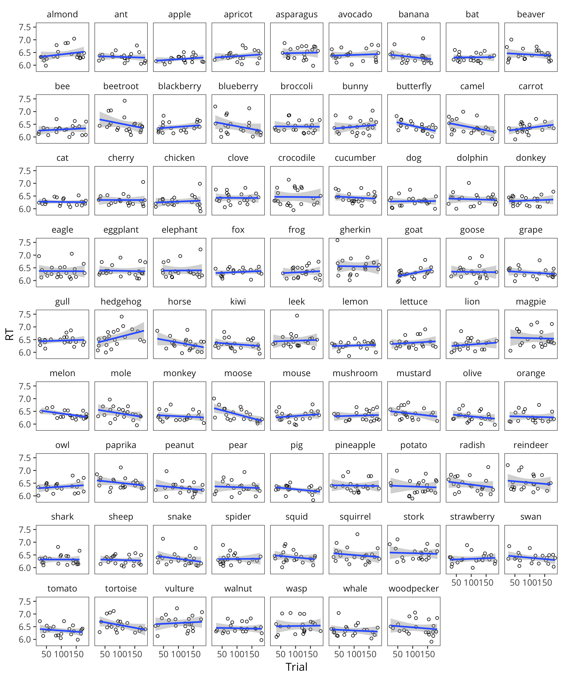
We’re going to have to change our generative process for our data, such that the generative process generates datapoints that are correlated within subject and within item.
trial_lm <- lm(RT ~ Trial, data = lexdec)
summary(trial_lm)
##
## Call:
## lm(formula = RT ~ Trial, data = lexdec)
##
## Residuals:
## Min 1Q Median 3Q Max
## -0.53961 -0.16943 -0.04366 0.11594 1.18357
##
## Coefficients:
## Estimate Std. Error t value Pr(>|t|)
## (Intercept) 6.4172041 0.0144549 443.948 <2e-16 ***
## Trial -0.0003060 0.0001256 -2.435 0.015 *
## ---
## Signif. codes: 0 '***' 0.001 '**' 0.01 '*' 0.05 '.' 0.1 ' ' 1
##
## Residual standard error: 0.2412 on 1657 degrees of freedom
## Multiple R-squared: 0.003567, Adjusted R-squared: 0.002965
## F-statistic: 5.931 on 1 and 1657 DF, p-value: 0.01498Previously we had: \[ y_i \sim \mathcal{N}(\mu_i, \sigma) \] \[ \mu_i = \beta_0 + \beta_1 \cdot x_{1_i} + \beta_2 \cdot x_{2_i} + \beta_3 \cdot x_{1_i} \cdot x_{2_i} \]
Now let’s incorporate the fact that each subject and each item has its own mean.
\[ y_i \sim \mathcal{N}(\mu_i, \sigma) \] \[ \mu_i = \beta_0 + \gamma_{s_i} + \gamma_{j_i} + ... \]
So the intercept for a particular datapoint will not just be \(\beta_0\), but rather \(\beta_0\) plus \(\gamma_s\) for the particular subject, plus \(\gamma_j\) for the particular item. So now we have incorporated different intercepts for different subjects and items in our model. We need to take one more step.
In general, while we know there is variation between subjects and items, we don’t think that variation is without bound. We think most subject means will be around the same, and most item means will be around the same.
So instead of just having these numbers here, let’s draw these numbers from a normal distribution:
\[ y_i \sim \mathcal{N}(\mu_i, \sigma) \] \[ \mu_i = \beta_0 + \gamma_{s_i} + \gamma_{j_i} + ... \] \[ \gamma_{s_i} \sim \mathcal{N}(0, \sigma_s) \] \[ \gamma_{j_i} \sim \mathcal{N}(0, \sigma_j) \]
This says the value of \(\gamma_{s_i}\) is probably 0, and with some probability as determined by the normal distribution it is some other value with some distance from 0.
\(\gamma_{s_i}\) is the extent to which the intercept for subject will differ from the mean intercept of all subjects.
Then we generate a \(\gamma_{j_i}\) for an item. Then we generate our data from a normal distribution around that mean.
Random intercepts
library(lme4)
library(lmerTest)

subject_lmer <- lmer(RT ~ Trial + (1 | Subject), data = lexdec)
summary(subject_lmer)
## Linear mixed model fit by REML t-tests use Satterthwaite approximations
## to degrees of freedom [lmerMod]
## Formula: RT ~ Trial + (1 | Subject)
## Data: lexdec
##
## REML criterion at convergence: -720.2
##
## Scaled residuals:
## Min 1Q Median 3Q Max
## -2.2919 -0.6592 -0.1547 0.4585 5.9198
##
## Random effects:
## Groups Name Variance Std.Dev.
## Subject (Intercept) 0.02362 0.1537
## Residual 0.03565 0.1888
## Number of obs: 1659, groups: Subject, 21
##
## Fixed effects:
## Estimate Std. Error df t value Pr(>|t|)
## (Intercept) 6.410e+00 3.540e-02 2.390e+01 181.06 <2e-16 ***
## Trial -2.348e-04 9.866e-05 1.637e+03 -2.38 0.0174 *
## ---
## Signif. codes: 0 '***' 0.001 '**' 0.01 '*' 0.05 '.' 0.1 ' ' 1
##
## Correlation of Fixed Effects:
## (Intr)
## Trial -0.292subject_item_lmer <- lmer(RT ~ Trial + (1 | Subject) + (1 | Word), data = lexdec)
summary(subject_item_lmer)## Linear mixed model fit by REML t-tests use Satterthwaite approximations
## to degrees of freedom [lmerMod]
## Formula: RT ~ Trial + (1 | Subject) + (1 | Word)
## Data: lexdec
##
## REML criterion at convergence: -889.2
##
## Scaled residuals:
## Min 1Q Median 3Q Max
## -2.2877 -0.6281 -0.1255 0.4695 5.9639
##
## Random effects:
## Groups Name Variance Std.Dev.
## Word (Intercept) 0.005917 0.07692
## Subject (Intercept) 0.023688 0.15391
## Residual 0.029727 0.17242
## Number of obs: 1659, groups: Word, 79; Subject, 21
##
## Fixed effects:
## Estimate Std. Error df t value Pr(>|t|)
## (Intercept) 6.410e+00 3.623e-02 2.620e+01 176.917 <2e-16 ***
## Trial -2.421e-04 9.144e-05 1.580e+03 -2.647 0.0082 **
## ---
## Signif. codes: 0 '***' 0.001 '**' 0.01 '*' 0.05 '.' 0.1 ' ' 1
##
## Correlation of Fixed Effects:
## (Intr)
## Trial -0.265So in addition to the fixed effects you see random effects! Fixed effects are the things we care about / that we are testing, generally.
ranef(subject_item_lmer)## $Word
## (Intercept)
## almond 0.038998545
## ant -0.048715756
## apple -0.111327213
## apricot -0.016836405
## asparagus 0.080002864
## avocado 0.012958691
## banana -0.055192917
## bat -0.064082218
## beaver 0.027394903
## bee -0.070003984
## beetroot 0.089689391
## blackberry 0.007068003
## blueberry 0.026381559
## broccoli 0.019879008
## bunny 0.020418217
## butterfly 0.018398728
## camel -0.001116122
## carrot -0.030619039
## cat -0.094408602
## cherry -0.033086956
## chicken -0.082120656
## clove 0.032575652
## crocodile 0.061636128
## cucumber 0.043826303
## dog -0.072658123
## dolphin -0.011186172
## donkey -0.054351097
## eagle -0.013678223
## eggplant -0.002950055
## elephant 0.009218789
## fox -0.043156871
## frog -0.037719537
## gherkin 0.139590239
## goat -0.090630150
## goose -0.037525696
## grape -0.063308841
## gull 0.059116314
## hedgehog 0.144568903
## horse -0.036221496
## kiwi -0.056176579
## leek 0.056788747
## lemon -0.094175390
## lettuce -0.008963495
## lion -0.069550247
## magpie 0.138014513
## melon -0.006588214
## mole 0.024069355
## monkey -0.063201725
## moose -0.014467843
## mouse -0.053501837
## mushroom -0.035372764
## mustard 0.023579443
## olive -0.072606788
## orange -0.079975735
## owl -0.023125267
## paprika 0.096982670
## peanut -0.066236199
## pear -0.038976821
## pig -0.103949904
## pineapple 0.014196533
## potato -0.017660621
## radish 0.048778101
## reindeer 0.114399282
## shark -0.055372672
## sheep -0.069741615
## snake -0.036911279
## spider -0.040257883
## squid 0.017186432
## squirrel 0.085250595
## stork 0.145771040
## strawberry -0.030711290
## swan -0.004613278
## tomato -0.034685487
## tortoise 0.143088886
## vulture 0.214216267
## walnut 0.042359430
## wasp 0.117086505
## whale -0.027202909
## woodpecker 0.061431940
##
## $Subject
## (Intercept)
## A1 -0.10560879
## A2 -0.16253238
## A3 0.01220767
## C -0.06219225
## D 0.01989228
## I -0.12986355
## J -0.12723174
## K -0.18828213
## M1 -0.20818866
## M2 0.14505662
## P 0.04260464
## R1 -0.07501217
## R2 0.08476099
## R3 0.00732681
## S -0.01056243
## T1 -0.02366095
## T2 0.41490299
## V 0.19846952
## W1 -0.11920960
## W2 0.07585889
## Z 0.21126425lmer_augmented <- augment(subject_item_lmer)
ggplot(lmer_augmented, aes(x = Trial)) +
geom_point(aes(y = .fitted, colour = Subject), shape = 1) +
geom_point(aes(y = .fixed), colour = "red")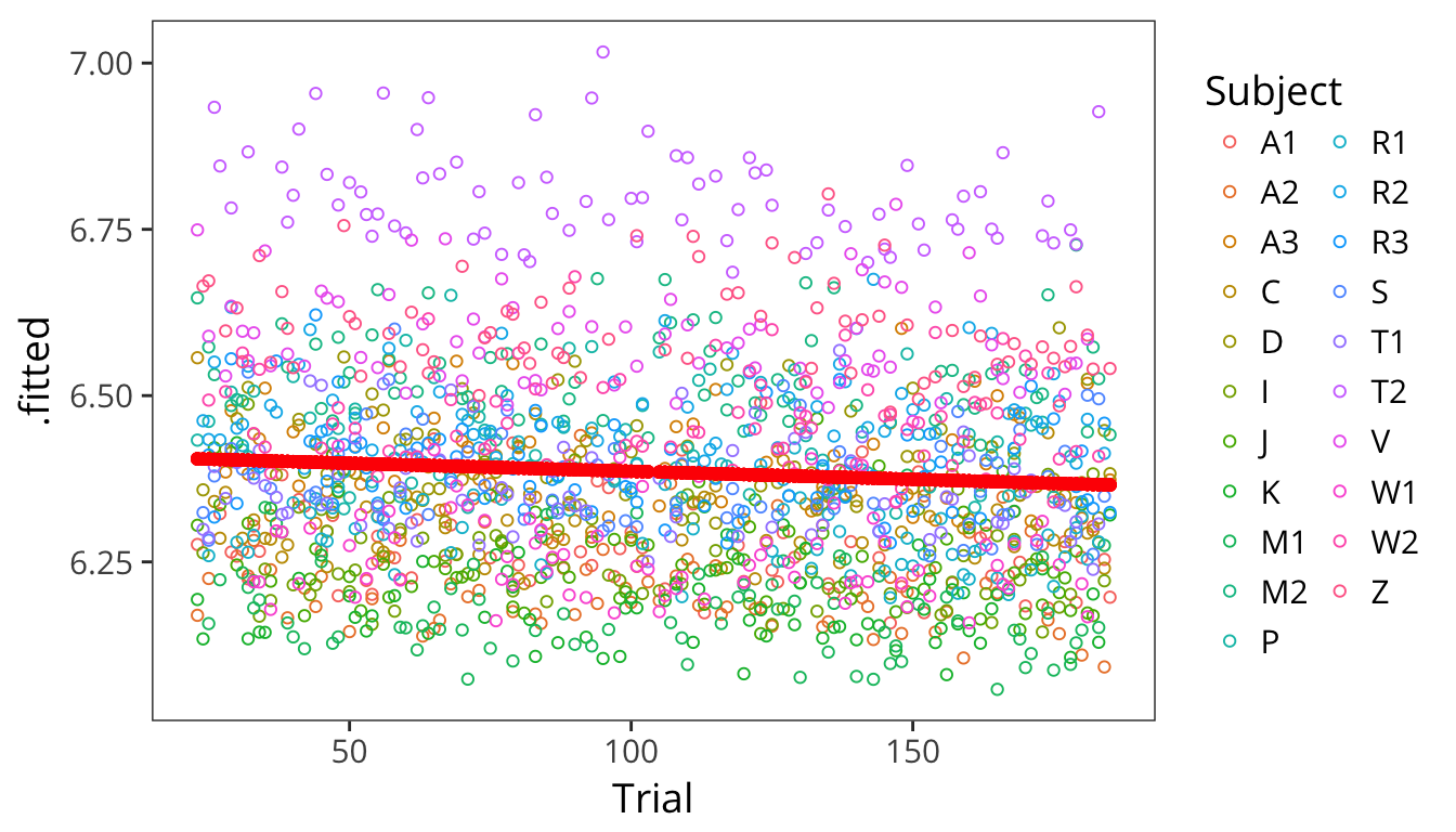
ggplot(lmer_augmented, aes(x = Trial)) +
  facet_wrap(~Subject) +
  geom_point(aes(y = .fitted, colour = Subject), shape = 1) +
  geom_point(aes(y = .fixed), colour = "red")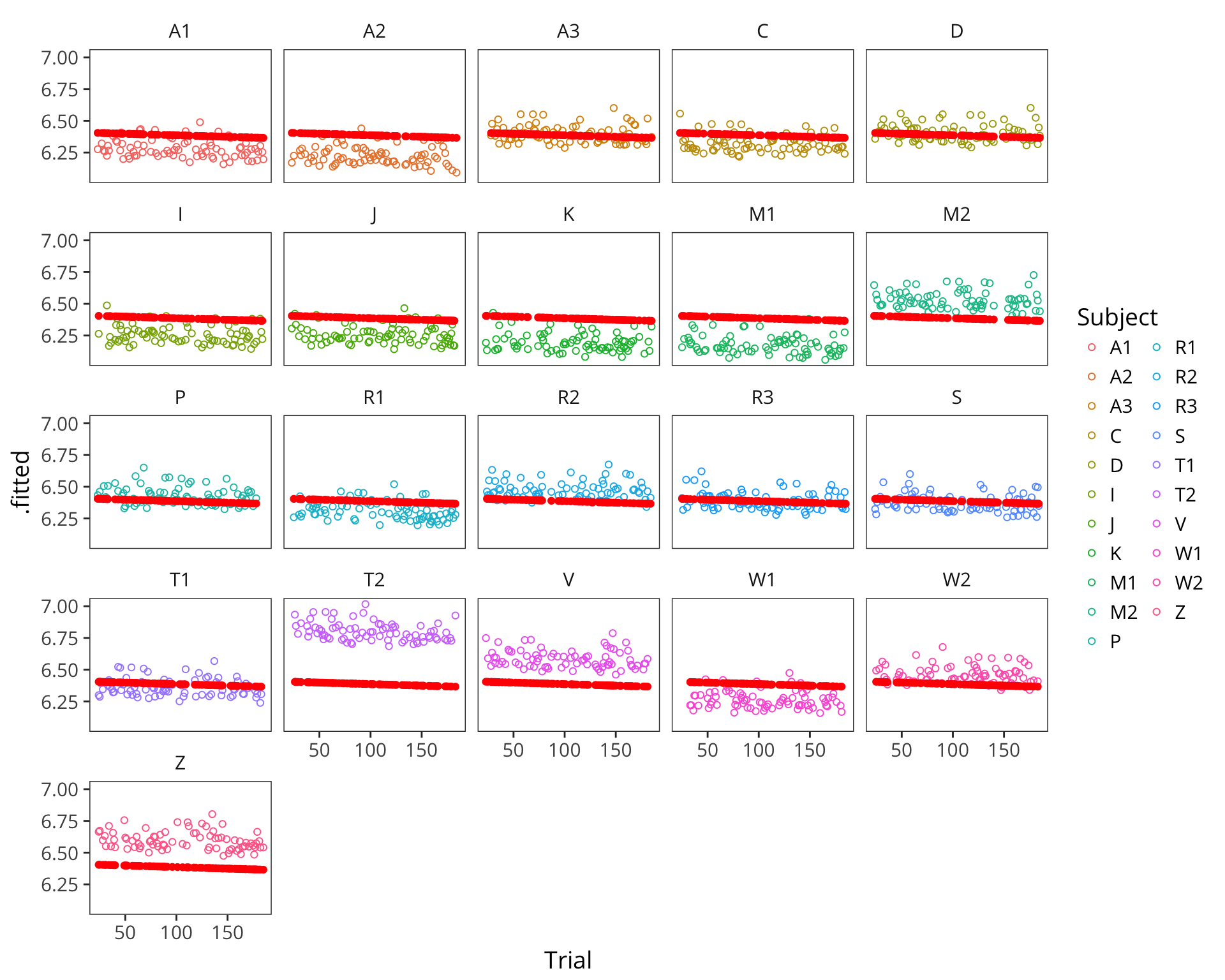
This kind of model is called a mixed effects regression with random intercepts. Our old coefficients here are called fixed effects because they are fixed in value across all datapoints. Our new coefficients \(\gamma\) are called random effects because they are drawn for each subject and item randomly from a normal distribution.
Random slopes
But you may find that not only do subjects and items have baseline differences, they may also be differentially affected by your experimental manipulation.
ggplot(lexdec, aes(x = Trial, y = RT)) +
  geom_smooth(aes(colour = Word), method = "lm", se = FALSE, size = 0.5) +
  geom_smooth(method = "lm", se = FALSE, color = "black") +
  scale_color_discrete(guide = FALSE)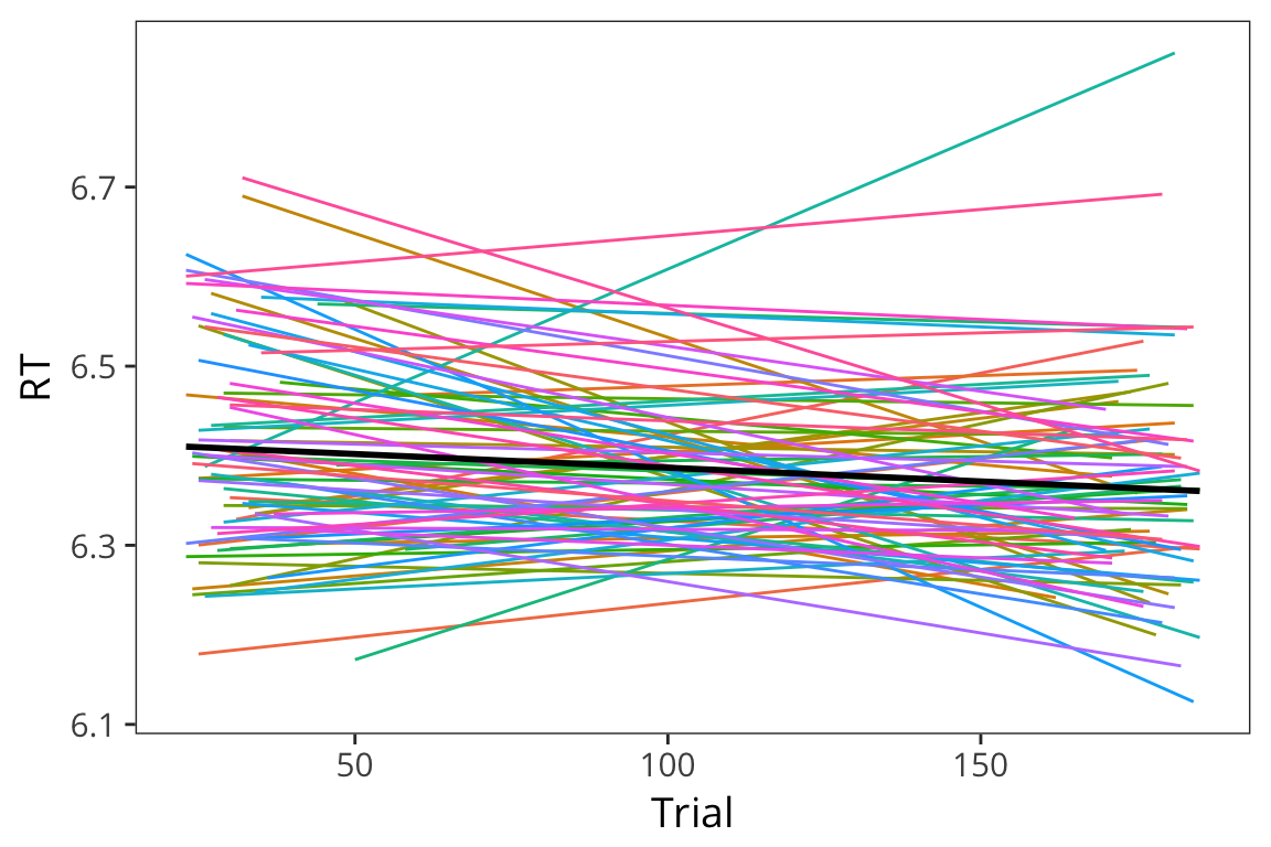
ggplot(lexdec, aes(x = Trial, y = RT)) +
  geom_smooth(aes(colour = Subject), method = "lm", se = FALSE, size = 0.5) +
  geom_smooth(method = "lm", se = FALSE, color = "black") +
  scale_color_discrete(guide = FALSE)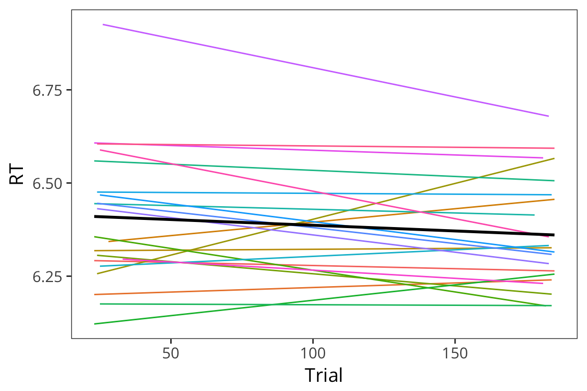
In these cases you can run mixed effects regression with random slopes. Here is the syntax for adding slopes:
slopes_lmer <- lmer(RT ~ Trial + (Trial | Subject) + (Trial | Word),
                    data = lexdec)
Sometimes lmer will fail to find a good set of parameter values for you. The first things to try in these cases is to double-check that your model formula is correct and then to scale any continuous predictors.
lexdec_scaled <- lexdec %>%
  mutate(Trial = scale(Trial))

slopes_lmer <- lmer(RT ~ Trial + (Trial | Subject) + (Trial | Word),
                    data = lexdec_scaled)
summary(slopes_lmer)
## Linear mixed model fit by REML t-tests use Satterthwaite approximations
## to degrees of freedom [lmerMod]
## Formula: RT ~ Trial + (Trial | Subject) + (Trial | Word)
## Data: lexdec_scaled
##
## REML criterion at convergence: -927
##
## Scaled residuals:
## Min 1Q Median 3Q Max
## -2.3633 -0.6100 -0.0973 0.4655 6.0248
##
## Random effects:
## Groups Name Variance Std.Dev. Corr
## Word (Intercept) 5.946e-03 0.077109
## Trial 2.069e-06 0.001438 -1.00
## Subject (Intercept) 2.366e-02 0.153824
## Trial 1.094e-03 0.033071 -0.31
## Residual 2.869e-02 0.169377
## Number of obs: 1659, groups: Word, 79; Subject, 21
##
## Fixed effects:
## Estimate Std. Error df t value Pr(>|t|)
## (Intercept) 6.385124 0.034920 22.680000 182.851 <2e-16 ***
## Trial -0.011506 0.008374 19.764000 -1.374 0.185
## ---
## Signif. codes: 0 '***' 0.001 '**' 0.01 '*' 0.05 '.' 0.1 ' ' 1
##
## Correlation of Fixed Effects:
## (Intr)
## Trial -0.259There are also some other tricks to try. If you can’t get it converge, it often means that you do not have enough data to fit all the parameters you are looking for. This is not great but there’s a semi-reasonable (or at least this is currently the best approach we’ve got) way to deal with it. You take out terms from the random effects structure in stepwise fashion until the model converges.
You can also model binary variables with mixed-effects models using glmer() and the family="binomial" argument.
Great visualization of mixed effects modeling: http://mfviz.com/hierarchical-models/
More information on glmm models: http://bbolker.github.io/mixedmodels-misc/glmmFAQ.html#model-specification