Continued introduction to ArcMap - editing and analyzing rasters and shapefiles

What we want to do here is to make our first map. Using remote sensing data for the Big Maria Mountains in SE California, we'll draw the contact between alluvium (recently deposited river sediments) and exposed bedrock. You'll get to perform a simple DEM analysis as well as create and edit a shapefile.

Step One -

In ArcMap open bigmarias.mxd. It's located at \\Langtang\public\fieldcamp2005\bigmarias\bigmarias.mxd

I've been so gracious as to collect a bunch of (free) remote sensing data for this area. You have at your disposal USGS topographic maps, DEMs (digital elevation models) at 10m where I can find it and at 30m everywhere else, color aerial photographs and Landsat satellite imagery. For your information, this data came from http://gis.ca.gov and there's more there...

Step Two -

You'll find that for this exercise, the DEMs and color photos are the most helpful. In fact, the DEMs are even more helpful if you use them to create a slope map. Since exposed bedrock often creates steeper slopes than alluvium, we can try and trace the break in slope to map the bedrock/alluvium contact. So, make a slope map from the two DEMs in ArcMap.

For instructions on doing this, click here.

Step Three -

You need to create a new shapefile to represent your bedrock/alluvium contact. To do this you need ArcCatalog. It can be opened by clicking the file cabinet button in the ArcMap window, or through the Start Menu.

A note on ArcCatalog - There is one important thing you should know. GIS data (shapefiles, coverages, rasters, etc.) actually consists of a number of different files, which you can see in the Windows Explorer. Because there are a number of files, and because you never quite know which files are important, you should only move GIS data around on the computer using ArcCatalog, which will always move everything you need.

There are three different types of shapefiles - point, polyline and polygon. The type of data each contains is evident from its name. So, for this exercise, where we will be drawing a line, we will want to create a polyline shapefile. Go for it.

For instructions on creating a shapefile, click here

Step Four -

Make sure you've added the new shapefile to the map. Now you need to edit that shapefile in order to add data to it.

Here's the lowdown on editing shapefiles

Step Five -

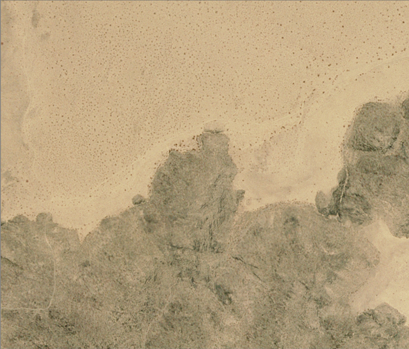
Now we're ready to draw a new line, following what we think to be the contact between alluvium and bedrock. Again, your best tools will be the slope maps you made, and especially the color aerial photographs. In the slope maps, you'll see that alluvium tends to form shallow slopes, while bedrock will tend to be exposed on steeper mountain sides. I'd suggest starting on the northeastern edge of the range. Here, you can see a distinct difference between the sandy, unconsolidated alluvium and the darker outcrop.

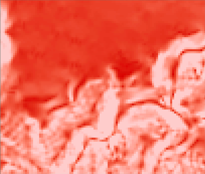
Also, this is where we have 10m DEM data. It should quickly become apparent that even with the 10 m data it is difficult to pin down the precise location of the contact. For instance, here's the 10 m slope map we made, at the same location, same scale as the aerial photo above. While you can see that there is a break in slope where the bedrock meets the alluvium, the data is too coarse to be of much good.

That being said, start drawing the contact!

For more instruction on how to make a line, click here

You may find that you want to snap new lines to old ones that you've already drawn.

Snapping instructions are here

Step Six -

Save your work! Make sure to save your edits before closing your editing session, and make sure to save your map file.

Added Bonus -

What's this? You don't like your line because it's so sharp and gross looking? There are ways to smooth the line.

Instructions for doing so are here