Lab 1

In this lab, we’ll try to cover some of the basic ways of interacting with R and then pretty quickly switch to data wrangling and data visualization.

Calculator

First of all, R can be used as a calculator:

1 + 1

## [1] 2

2 * 3

## [1] 6

3 ^ 2

## [1] 9

5 %% 3

## [1] 2

It’s a good idea not to work directly in the console but to have a script where you will first write your commands and then execute them in the console. Once you open a new R script there are a few useful things to note:

Use # to comment lines so they don’t get executed
You can send a line directly to console from script with command + return (on mac) or ctrl + enter (windows)

Variables

Values can be stored as variables

a <- 2
a

## [1] 2

b <- 2 + 2
b

## [1] 4

c <- b + 3
c

## [1] 7

When you’re defining variables, try to use meaningful names like average_of_ratings rather than variable1.

Functions

A function is an object that takes some arguments and returns a value.

print("hello world")

## [1] "hello world"

sqrt(4)

## [1] 2

log(4)

## [1] 1.386294

abs(-4)

## [1] 4

?log

If you are ever unsure about how a function works or what arguments it takes. Typing ?[FUNCTION NAME GOES HERE] will open up a help file (e.g., ?c).

A function takes certain arguments (inputs). These can be referenced by position or by name. Arguments can have default values that they take if you not specified. Arguments without defaults have to be specified. Argument values can be also be variables or expressions.

# log(x, base = exp(1))
log(4)

## [1] 1.386294

log(x = 4, base = 2)

## [1] 2

# log(base = 2)
a <- exp(1) ^ 5
log(a, base = exp(1))

## [1] 5

Vectors

If you want to store more than one thing in a variable you may want to make a vector. To do this you will use the function c() which combines values

v1 <- c(1, 2, 3, 4, 5, 6, 7, 8, 9, 10)
v1

##  [1]  1  2  3  4  5  6  7  8  9 10

Now that we have some values stored in a vector, we may want to access those values and we can do this by using their position in the vector or index.

v1[1]

## [1] 1

v1[5]

## [1] 5

v1[-1]

## [1]  2  3  4  5  6  7  8  9 10

v1[c(2, 7)]

## [1] 2 7

v1[-c(2, 7)]

## [1]  1  3  4  5  6  8  9 10

v1[1:3]

## [1] 1 2 3

v1[-(1:3)]

## [1]  4  5  6  7  8  9 10

You may also want to get some overall information about the vector:

what types of values are in v1?

str(v1)

##  num [1:10] 1 2 3 4 5 6 7 8 9 10

class(v1)

## [1] "numeric"

how long is v1?
```
length(v1)
```
```
## [1] 10
```
what is the average of all these values?
```
mean(v1)
```
```
## [1] 5.5
```
```
median(v1)
```
```
## [1] 5.5
```
what is the standard deviation of all these values?
```
sd(v1)
```
```
## [1] 3.02765
```

what is the range of these values?

min(v1)

## [1] 1

max(v1)

## [1] 10

range(v1)

## [1]  1 10

Earlier we created v1 by simply listing all the elements in it and usingc() but if you have lots of values, this is very tedious. There are some functions that can help make vectors more efficiently

v2 <- 1:10
v2

##  [1]  1  2  3  4  5  6  7  8  9 10

v3 <- rep(1, times = 10)
v3

##  [1] 1 1 1 1 1 1 1 1 1 1

v4 <- rep(1:2, 5)
v4

##  [1] 1 2 1 2 1 2 1 2 1 2

v5 <- rep(1:2, each = 5)
v5

##  [1] 1 1 1 1 1 2 2 2 2 2

v6 <- seq(from = 1, to = 20, by = 2)
v6

##  [1]  1  3  5  7  9 11 13 15 17 19

Note that for v4, I didn’t include the names of the arguments but R figures out which is which by the order

You can also apply operations to all elements of the vector simultaneously.

v1 + 1

##  [1]  2  3  4  5  6  7  8  9 10 11

v1 * 100

##  [1]  100  200  300  400  500  600  700  800  900 1000

You can also do pair-wise operations on 2 vectors.

v1 + v2

##  [1]  2  4  6  8 10 12 14 16 18 20

Characters

So far we’ve looked at numeric variables and vectors, but they can also be characters.

animal <- "dog"
animal

## [1] "dog"

pets <- c("dog", "cat", "hamster", "turtle")
pets

## [1] "dog"     "cat"     "hamster" "turtle"

str(pets)

##  chr [1:4] "dog" "cat" "hamster" "turtle"

You can even store numbers as strings (and sometimes data you load from a file will be stored this way so watch out for that)

some_numbers <- c("2", "3", "4")

…but you can’t manipulate them as numbers

some_numbers + 1

So you might want to convert the strings into numbers first using as.numeric()

some_numbers <- as.numeric(some_numbers)
some_numbers + 1

## [1] 3 4 5

Conversely, numeric vectors can be coerced into character vectors with as.character().

NA

Another important datatype is NA. Say I’m storing people’s heights in inches in a dataframe, but I don’t have data on the third person.

heights <- c(72, 70, NA, 64)
str(heights)

##  num [1:4] 72 70 NA 64

Even though it’s composed of letters, NA is not a string, in this case it’s numeric, and represents a missing value, or an invalid value, or whatever. You can still perform operations on the height vector:

heights + 1

## [1] 73 71 NA 65

heights * 2

## [1] 144 140  NA 128

if you had an NA in a vector of strings, its datatype would be a character.

pets <- c("dog", "cat", NA, "turtle")
str(pets)

##  chr [1:4] "dog" "cat" NA "turtle"

If you have NA in your vector and want to use a function on it, this can complicate things

mean(heights)

## [1] NA

To avoid returning NA, you may want to just throw out the NA values using na.omit and work with what’s left.

heights_no_NA <- na.omit(heights)
mean(heights_no_NA)

## [1] 68.66667

Alternatively, many functions have a built-in argument na.rm that you can use to tell the function what to do about NA values. So you can do the previous step in 1 line:

mean(heights_no_NA, na.rm = TRUE)

## [1] 68.66667

It can also be useful to know if a vector contains NA ahead of time and where those values are:

is.na(heights)

## [1] FALSE FALSE  TRUE FALSE

which(is.na(heights))

## [1] 3

Logicals

This brings us to another important datatype: logical They are TRUE or FALSE, or T or F. Here are some expressions that return logical values:

v <- 1:5
v == 2 # equal

## [1] FALSE  TRUE FALSE FALSE FALSE

v != 2 # not equal

## [1]  TRUE FALSE  TRUE  TRUE  TRUE

v > 2 # greater than

## [1] FALSE FALSE  TRUE  TRUE  TRUE

v >= 2 # greater than or equal to

## [1] FALSE  TRUE  TRUE  TRUE  TRUE

v < 2 # less than

## [1]  TRUE FALSE FALSE FALSE FALSE

v <= 2 # less than or equal to

## [1]  TRUE  TRUE FALSE FALSE FALSE

v > 2 & v != 4 # and

## [1] FALSE FALSE  TRUE FALSE  TRUE

v > 2 | v == 1 # or

## [1]  TRUE FALSE  TRUE  TRUE  TRUE

v_2 <- v > 2
str(v_2)

##  logi [1:5] FALSE FALSE TRUE TRUE TRUE

v[v_2]

## [1] 3 4 5

v[v > 2]

## [1] 3 4 5

as.numeric(v_2)

## [1] 0 0 1 1 1

Try it yourself…

Make a vector, “tens” of all the multiples of 10 up to 200.

Find the indices of the numbers divisible by 3

tens <- seq(from = 10, to = 200, by = 10)
tens

##  [1]  10  20  30  40  50  60  70  80  90 100 110 120 130 140 150 160 170
## [18] 180 190 200

which(tens %% 3 == 0)

## [1]  3  6  9 12 15 18

Dataframes

Most data you will work with in R will be in a dataframe format. Dataframes are basically tables where each column is a vector with a name. Dataframes can combine character vectors, numeric vectors, logical vectors, etc. This is really useful for data from experiments where you may want one column to contain information about the name of the condition (a string) and another column to contain response times (a number).

Let’s read in some data!

But first a digression… One of the best things about R is that it is open-source and lots of R users who find that some functionality is missing from base R (which is what we’ve been using so far) will write their own functions and then share them with the R community. Often times they’ll write whole packages of functions to greatly enhance the capabilities of base R. In order for you to use those packages, they need to be installed on your computer and loaded up in your current session. For current purposes, you will need the tidyverse package and you can install it with this simple command:

install.packages("tidyverse")

When the installation is done, load up the library of functions in the package with the following command:

library(tidyverse)

Okay, digression over.

Let’s read in your lexical decision data from earlier using a tidyverse function called read_csv(). You can read data from the web or locally relative to your working directory. Change your working directory by clicking on Session > Set Working Directory in the menu up top.

data_source <- "http://web.mit.edu/psycholinglab/www/data/"
rt_data <- read_csv(file.path(data_source, "in_lab_rts_2020.csv"))

Our data is now stored as a dataframe. The output message tells us what datatype read_csv() assigned to every column. It usually does a pretty good job of guessing the appropriate datatype but on occasion you may have to correct using a function like as.numeric() or as.character().

Note that the path to the data can be any folder on your computer or online (a url). If you just put in the filename without the path, it will look for the file in the local folder.

Also note, that if you have column headers in your csv file, read_csv() will automatically name your columns accordingly and you won’t have to specify col_names=.

At this point, it’s a good idea to look at your data to make sure everything was correctly uploaded. In RStudio, you can open up a viewing pane with the command View(d) to see the data in spreadsheet form (or command + click on the variable). You can also use summary(), str() and glimpse()

rt_data

## # A tibble: 310 x 5
##             time subject word       trial    rt
##            <dbl>   <dbl> <chr>      <dbl> <dbl>
##  1 1581099326101       2 book           0 1.12 
##  2 1581099327976       2 noosin         1 0.874
##  3 1581099328278       4 book           0 0.806
##  4 1581099329608       2 eat            2 0.630
##  5 1581099330387       4 noosin         1 1.11 
##  6 1581099331277       6 book           0 2.96 
##  7 1581099331545       2 goamboozle     3 0.936
##  8 1581099332055       4 eat            2 0.667
##  9 1581099332134       1 book           0 2.34 
## 10 1581099333304       5 book           0 1.62 
## # … with 300 more rows

You can also extract just the names of the columns:

names(rt_data)

## [1] "time"    "subject" "word"    "trial"   "rt"

Or just the first (or last) few rows of the dataframe:

head(rt_data)

## # A tibble: 6 x 5
##            time subject word   trial    rt
##           <dbl>   <dbl> <chr>  <dbl> <dbl>
## 1 1581099326101       2 book       0 1.12 
## 2 1581099327976       2 noosin     1 0.874
## 3 1581099328278       4 book       0 0.806
## 4 1581099329608       2 eat        2 0.630
## 5 1581099330387       4 noosin     1 1.11 
## 6 1581099331277       6 book       0 2.96

tail(rt_data)

## # A tibble: 6 x 5
##            time subject word           trial       rt
##           <dbl>   <dbl> <chr>          <dbl>    <dbl>
## 1 1581099590101      18 three             17 0.725   
## 2 1581099591802      18 seefer            18 0.699   
## 3 1581099593568      18 sqw               19 0.764   
## 4 1581099595317      18 encyclopedia      20 0.748   
## 5 1581099597181      18 understandable    21 0.862   
## 6 1581099614285      19 book               0 0.000924

Or look at the dimensions of your dataframe

nrow(rt_data)

## [1] 310

ncol(rt_data)

## [1] 5

To access a specific column, row, or cell you can use indexing in much the same way you can with vectors (just now with 2 dimensions)

rt_data[1, 2] # what's in the 1st row, 2nd column

## # A tibble: 1 x 1
##   subject
##     <dbl>
## 1       2

rt_data[1, ] # the 1st row for all columns

## # A tibble: 1 x 5
##            time subject word  trial    rt
##           <dbl>   <dbl> <chr> <dbl> <dbl>
## 1 1581099326101       2 book      0  1.12

rt_data[, 2] # all rows for the 2nd column

## # A tibble: 310 x 1
##    subject
##      <dbl>
##  1       2
##  2       2
##  3       4
##  4       2
##  5       4
##  6       6
##  7       2
##  8       4
##  9       1
## 10       5
## # … with 300 more rows

rt_data[, c(2, 5)] # all rows for columns 2 and 5

## # A tibble: 310 x 2
##    subject    rt
##      <dbl> <dbl>
##  1       2 1.12 
##  2       2 0.874
##  3       4 0.806
##  4       2 0.630
##  5       4 1.11 
##  6       6 2.96 
##  7       2 0.936
##  8       4 0.667
##  9       1 2.34 
## 10       5 1.62 
## # … with 300 more rows

rt_data[, c("subject", "rt")]

## # A tibble: 310 x 2
##    subject    rt
##      <dbl> <dbl>
##  1       2 1.12 
##  2       2 0.874
##  3       4 0.806
##  4       2 0.630
##  5       4 1.11 
##  6       6 2.96 
##  7       2 0.936
##  8       4 0.667
##  9       1 2.34 
## 10       5 1.62 
## # … with 300 more rows

Another easy way to extract a dataframe column is by using the $ operator and the column name

head(rt_data$rt)

## [1] 1.1210220 0.8742580 0.8055780 0.6304672 1.1081619 2.9571130

rt_data$rt is a (numeric) vector so you can perform various operations on it (as we saw earlier)

head(rt_data$rt * 2)

## [1] 2.242044 1.748516 1.611156 1.260934 2.216324 5.914226

mean(rt_data$rt)

## [1] 0.9499523

Data manipulation (`dplyr`)

Often when you upload data it’s not yet in a convenient, “tidy” form so data wrangling refers to the various cleaning and re-arranging steps between uploading data and being able to visualize or analyze it. I’ll start out by showing you a few of the most common things you might want to do with your data.

For example, in this dataset, we want to know about how response times on the lexical decision task might differ depending on whether it’s a real word or a non-word but this information is missing from our data.

Let’s see what words were included in the experiment.

words <- unique(rt_data$word)
words

##  [1] "book"             "noosin"           "eat"             
##  [4] "goamboozle"       "condition"        "xdqww"           
##  [7] "word"             "retire"           "feffer"          
## [10] "fly"              "qqqwqw"           "coat"            
## [13] "condensationatee" "sporm"            "art"             
## [16] "goam"             "gold"             "three"           
## [19] "seefer"           "sqw"              "encyclopedia"    
## [22] "understandable"

Now let’s make a vector containing only the real words:

real_words <- words[c(1, 3, 5, 7, 8, 10, 12, 15, 17, 18, 21, 22)]
real_words

##  [1] "book"           "eat"            "condition"      "word"          
##  [5] "retire"         "fly"            "coat"           "art"           
##  [9] "gold"           "three"          "encyclopedia"   "understandable"

`mutate`

Now we can add a column to our dataframe, rt_data, that contains that condition information. We’re going to do this using the mutate() function.

We can check if a value is represented in an array using the operator %in%.

"cat" %in% c("cat", "dog", "hamster")

## [1] TRUE

c("cat", "ocelot") %in% c("cat", "dog", "hamster")

## [1]  TRUE FALSE

rt_data <- mutate(rt_data, is_real = word %in% real_words)
head(rt_data)

## # A tibble: 6 x 6
##            time subject word   trial    rt is_real
##           <dbl>   <dbl> <chr>  <dbl> <dbl> <lgl>  
## 1 1581099326101       2 book       0 1.12  TRUE   
## 2 1581099327976       2 noosin     1 0.874 FALSE  
## 3 1581099328278       4 book       0 0.806 TRUE   
## 4 1581099329608       2 eat        2 0.630 TRUE   
## 5 1581099330387       4 noosin     1 1.11  FALSE  
## 6 1581099331277       6 book       0 2.96  TRUE

mutate() is extremely useful anytime you want to add information to your data. For instance, the reaction times here appear to be in seconds but maybe we want to look at them in milliseconds. Maybe we also want to code if the word starts with the letter “b” and code which words are longer than 6 letters long. This can be done all at once.

mutate(rt_data,
       rt_ms = rt * 1000,
       starts_d = str_sub(word, 1, 1) == "b",
       longer_than_6 = if_else(str_length(word) > 6, "long", "short"))

## # A tibble: 310 x 9
##         time subject word  trial    rt is_real rt_ms starts_d longer_than_6
##        <dbl>   <dbl> <chr> <dbl> <dbl> <lgl>   <dbl> <lgl>    <chr>        
##  1   1.58e12       2 book      0 1.12  TRUE    1121. TRUE     short        
##  2   1.58e12       2 noos…     1 0.874 FALSE    874. FALSE    short        
##  3   1.58e12       4 book      0 0.806 TRUE     806. TRUE     short        
##  4   1.58e12       2 eat       2 0.630 TRUE     630. FALSE    short        
##  5   1.58e12       4 noos…     1 1.11  FALSE   1108. FALSE    short        
##  6   1.58e12       6 book      0 2.96  TRUE    2957. TRUE     short        
##  7   1.58e12       2 goam…     3 0.936 FALSE    936. FALSE    long         
##  8   1.58e12       4 eat       2 0.667 TRUE     667. FALSE    short        
##  9   1.58e12       1 book      0 2.34  TRUE    2342. TRUE     short        
## 10   1.58e12       5 book      0 1.62  TRUE    1625. TRUE     short        
## # … with 300 more rows

Note: + str_sub() extracts a subset of word starting at position 1 and ending at position 1 (i.e., just the first letter). + if_else() is a useful function which takes a logical comparison as a first argument and then what to do if it is TRUE as the second argument and what to do if it is FALSE as the third.

`filter`

Now let’s say we want to look at only a subset of the data, we can filter() it:

filter(rt_data, str_length(word) > 6)

## # A tibble: 70 x 6
##             time subject word       trial    rt is_real
##            <dbl>   <dbl> <chr>      <dbl> <dbl> <lgl>  
##  1 1581099331545       2 goamboozle     3 0.936 FALSE  
##  2 1581099333536       2 condition      4 0.989 TRUE   
##  3 1581099333782       4 goamboozle     3 0.726 FALSE  
##  4 1581099335315       4 condition      4 0.532 TRUE   
##  5 1581099336832       6 goamboozle     3 0.697 FALSE  
##  6 1581099338916       6 condition      4 1.08  TRUE   
##  7 1581099339228       1 goamboozle     3 1.05  FALSE  
##  8 1581099340671       5 goamboozle     3 1.93  FALSE  
##  9 1581099341640       3 goamboozle     3 0.872 FALSE  
## 10 1581099342420       5 condition      4 0.747 TRUE   
## # … with 60 more rows

`select`

If your dataframe is getting unruly, you can focus on a few key columns with select()

select(rt_data, subject, word, rt)

## # A tibble: 310 x 3
##    subject word          rt
##      <dbl> <chr>      <dbl>
##  1       2 book       1.12 
##  2       2 noosin     0.874
##  3       4 book       0.806
##  4       2 eat        0.630
##  5       4 noosin     1.11 
##  6       6 book       2.96 
##  7       2 goamboozle 0.936
##  8       4 eat        0.667
##  9       1 book       2.34 
## 10       5 book       1.62 
## # … with 300 more rows

`arrange`

You can also sort the dataframe by one of the columns:

arrange(rt_data, rt)

## # A tibble: 310 x 6
##             time subject word      trial       rt is_real
##            <dbl>   <dbl> <chr>     <dbl>    <dbl> <lgl>  
##  1 1581099355362       7 fly           9 0.000146 TRUE   
##  2 1581099614285      19 book          0 0.000924 TRUE   
##  3 1581099354360       7 feffer        8 0.421    FALSE  
##  4 1581099513370      10 word          6 0.448    TRUE   
##  5 1581099516376      10 feffer        8 0.449    FALSE  
##  6 1581099349720       3 feffer        8 0.498    FALSE  
##  7 1581099350167       6 coat         11 0.498    TRUE   
##  8 1581099506583      10 eat           2 0.510    TRUE   
##  9 1581099500342      17 coat         11 0.517    TRUE   
## 10 1581099335315       4 condition     4 0.532    TRUE   
## # … with 300 more rows

`group_by` and `summarise`

Most of the time when you have data, the ultimate goal is to summarize it in some way. For example, you may want to know the mean response time for each subject by type of word (real vs. fake).

summarise(group_by(rt_data, subject, is_real), mean_rt = mean(rt))

## # A tibble: 30 x 3
##    subject is_real mean_rt
##      <dbl> <lgl>     <dbl>
##  1       1 FALSE     1.55 
##  2       1 TRUE      1.36 
##  3       2 FALSE     0.923
##  4       2 TRUE      0.790
##  5       3 FALSE     0.797
##  6       3 TRUE      0.706
##  7       4 FALSE     0.891
##  8       4 TRUE      0.861
##  9       5 FALSE     1.60 
## 10       5 TRUE      0.913
## # … with 20 more rows

As you can see, we often want to string tidyverse functions together which can get difficult to read. The solution to this is…

`%>%`

We can create a pipeline where the dataframe undergoes various transformations one after the other with the same functions, mutate(), filter(), etc. without having to repeat the name of the dataframe over and over and much more intuitive syntax.

rt_data %>%
  group_by(subject, is_real) %>%
  summarise(mean_rt = mean(rt))

## # A tibble: 30 x 3
##    subject is_real mean_rt
##      <dbl> <lgl>     <dbl>
##  1       1 FALSE     1.55 
##  2       1 TRUE      1.36 
##  3       2 FALSE     0.923
##  4       2 TRUE      0.790
##  5       3 FALSE     0.797
##  6       3 TRUE      0.706
##  7       4 FALSE     0.891
##  8       4 TRUE      0.861
##  9       5 FALSE     1.60 
## 10       5 TRUE      0.913
## # … with 20 more rows

And we can keep adding functions to the pipeline very easily…

rt_data %>%
  group_by(subject, is_real) %>%
  summarise(mean_rt = mean(rt)) %>%
  filter(mean_rt < 2)

## # A tibble: 30 x 3
##    subject is_real mean_rt
##      <dbl> <lgl>     <dbl>
##  1       1 FALSE     1.55 
##  2       1 TRUE      1.36 
##  3       2 FALSE     0.923
##  4       2 TRUE      0.790
##  5       3 FALSE     0.797
##  6       3 TRUE      0.706
##  7       4 FALSE     0.891
##  8       4 TRUE      0.861
##  9       5 FALSE     1.60 
## 10       5 TRUE      0.913
## # … with 20 more rows

We can look just at conditions and add some summary stats

rt_data %>%
  group_by(is_real) %>%
  summarise(mean_rt = mean(rt),
            median_rt = median(rt),
            sd_rt = sd(rt))

## # A tibble: 2 x 4
##   is_real mean_rt median_rt sd_rt
##   <lgl>     <dbl>     <dbl> <dbl>
## 1 FALSE     1.04      0.867 0.595
## 2 TRUE      0.878     0.748 0.499

It looks like average response time was longer for fake words.

Try it yourself…

Add a new column to rt_data that codes whether the word ends with “n”

Get the means and counts for real and fake words split by whether they end in “n” or not

rt_data_n <- rt_data %>%
  mutate(is_real = word %in% real_words) %>%
  mutate("ends_with_n" = str_sub(word, -1, -1) == "n") %>%
  group_by(is_real, ends_with_n) %>%
  summarise(mean_rt = mean(rt),
            n_rt = n())
rt_data_n

## # A tibble: 4 x 4
##   is_real ends_with_n mean_rt  n_rt
##   <lgl>   <lgl>         <dbl> <int>
## 1 FALSE   FALSE         1.02    126
## 2 FALSE   TRUE          1.19     14
## 3 TRUE    FALSE         0.864   156
## 4 TRUE    TRUE          1.04     14

Data visualization (`ggplot2`)

Looking at columns of numbers isn’t really the best way to do data analysis. You could be tripped up by placement of decimal points, you might accidentally miss a big number. It would be much better if we could PLOT these numbers so we can visually tell if anything stands out.

If you’ve taken an introductory Psych or Neuro course you might know that a huge proportion of human cortex is devoted to visual information processing; we have hugely powerful abilities to process visual data. By using plotting we can leverage that ability to get a fast sense of what is going on in our data.

Visualizing your data is an extremely important part of any data analysis. tidyverse contains a whole library of functions for plotting: ggplot2. I’ll be showing you how to use these functions but also I’ll be trying to give you some intuitions about how researchers use visualization to get a better understanding of their data.

The first thing you might want to know is what your dependent variable, in this case the response time, looks like. In other words, how is it distributed?

Histograms

ggplot(rt_data) +
  geom_histogram(aes(x = rt))

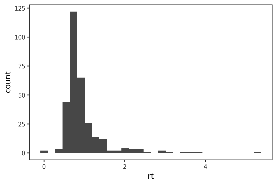
ggplot syntax might seem a little unusual. You can think of it as first creating a plot coordinate system with ggplot() and the you can add layers of information with +.

ggplot(data = rt_data) would create an empty plot because you haven’t told it anything about what variables you’re interested in or how you want to look at them. This is where geometric objects, or “geoms”, come in.

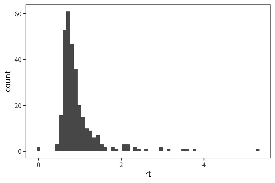
geom_histogram() is going to make this plot a histogram. A histogram has values of whatever variable you choose on the x axis and counts of those values on the y. The aesthetic mapping, aes(), arguments let us specify which variable, in this case rt, we want to know the distribution of. We can also change visual aspects of the geom, like the width of the bins, depending on what will make the graph more clear and informative.

ggplot(rt_data) +
  geom_histogram(aes(x = rt), bins = 60)

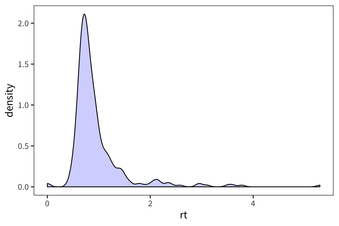
Another way to look at the distribution is to plot the density with geom_density()

ggplot(rt_data) +
  geom_density(aes(x = rt), fill = "blue", alpha = 0.2)

What can we learn from this histogram?

In this histogram we can see that there are a lot of response times around 1 second and a few longer outlier response times. This is important to know for when we analyze the response times because certain descriptive statistics like the mean are very sensitive to outliers.

Scatterplots

Let’s say we are curious to see if people speed up or slow down over the course of doing the lexical decision task. So, we want to plot trial number and compare it with mean rt. Let’s put trial number on the x axis, mean rt on the y axis, and make a scatterplot. For this we’re going to use a different geom, geom_point(). Contrary to geom_histogram() this takes a minimum of 2 arguments, x and y.

ggplot(rt_data) +
  geom_point(aes(x = trial, y = rt))

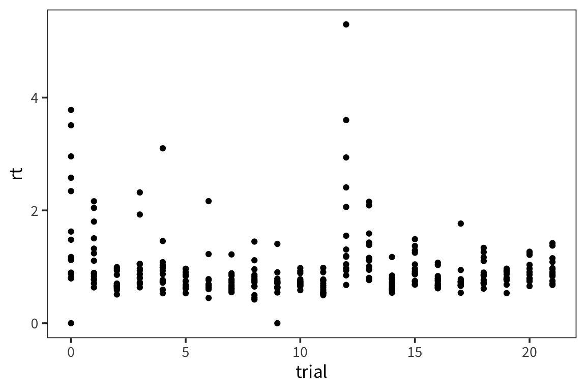
This is a fair number of data points so it’s a little difficult to see what’s going on. It might be useful to also show what the average across participants looks like at every timepoint. We can just add another layer to this same graph with the +, in this case we’ll use geom_line()

rt_by_trials <- rt_data %>%
  group_by(trial) %>%
  summarise(mean_rt = mean(rt))

ggplot() +
  geom_point(data = rt_data, aes(x = trial, y = rt), alpha = 0.2) +
  geom_line(data = rt_by_trials, aes(x = trial, y = mean_rt), color = "blue")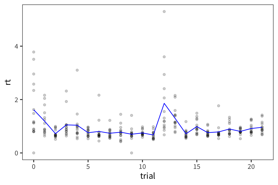

Because there were so many points and it was difficult to see, I made each point less opaque using alpha = 0.2 as an argument for geom_point() and I made the line connecting averages stand out by making it blue with color = "blue" as an argument to geom_line()
Note that I’m plotting 2 different datasets withing the same graph and this is easy to do because you can define data separately for each geom.

What can we learn from this scatterplot + line graph?

Is anything different happening in the first few trials? Does there seem to be a trend over the course of the trials?

Facets

What hypothesis do we want to test about the data? Maybe fake words take longer than real words to identify.

rt_data <- rt_data %>%
  mutate(word_type = if_else(is_real, "Real", "Fake"))

Now we want to start addressing our question about how RTs may differ for real vs. fake words. One way to do this is to split the RT data we have into Real and Fake and plot the data side by side. ggplot has an easy way to do that with facetting.

ggplot(rt_data) +
  geom_histogram(aes(x = rt), bins = 60, color = "white") +
  facet_wrap(vars(word_type))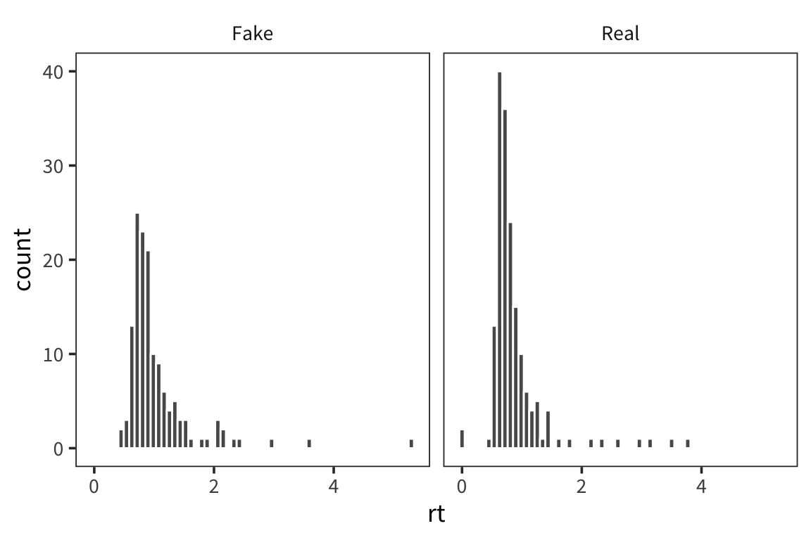

ggplot(rt_data) +
  geom_density(aes(x = rt), fill = "blue", alpha = 0.2) +
  facet_wrap(vars(word_type))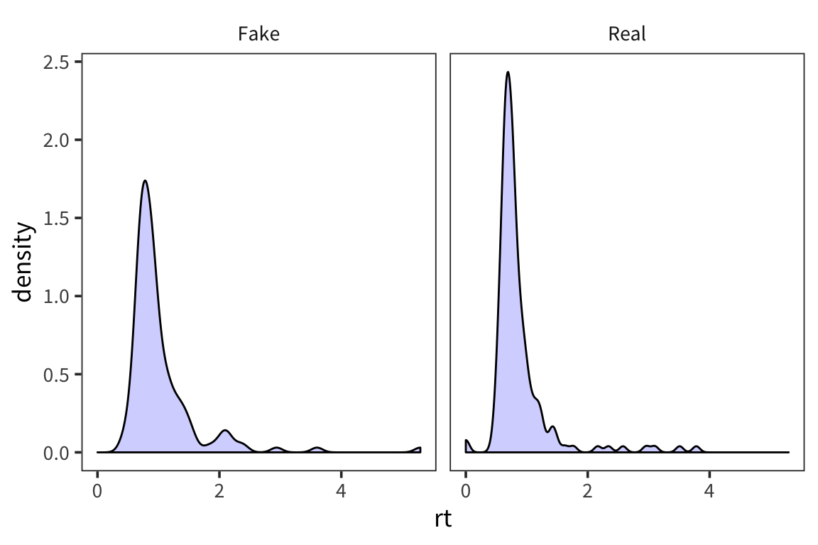

What do you observe?

This is informative but it’s not the easiest way to really draw a comparison in this case.

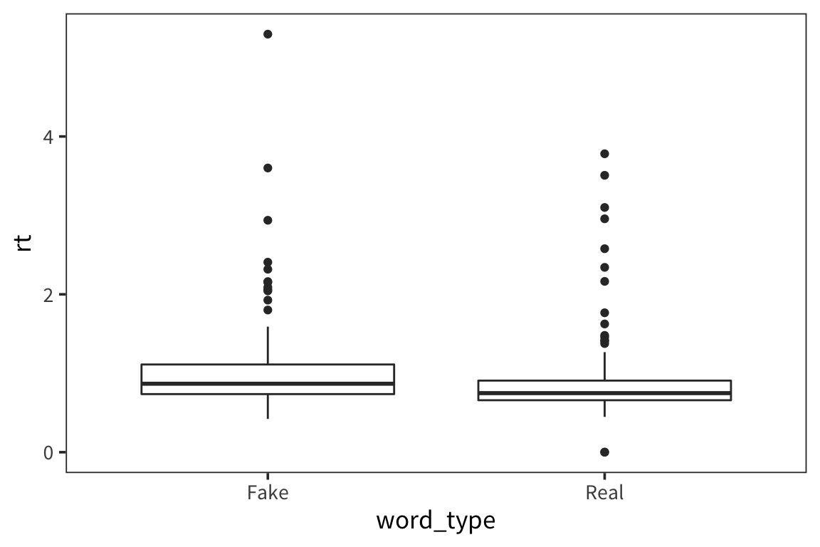
Boxplots

We want to aggregate the data but maintain some information about its variability. We can use a boxplot which plots the quartiles of the distribution (2^nd quartile = median).

ggplot(rt_data) +
  geom_boxplot(aes(x = word_type, y = rt))

Violin plots

Another, more aesthetically pleasing way to plot this is with violin plots

ggplot(rt_data) +
  geom_violin(aes(x = word_type, y = rt, fill = word_type))

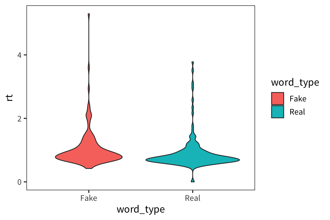
What can we learn from this boxplot?

It looks like real words have faster median RTs and somewhat less variability (except for that 1 outlier).

Barplots

Another commonly way to plot this is with a barplot. Bar plots are very popular possibly because they allow you to plot the mean which is a statistic that people find really useful, but they actually obscure a lot of information about the distribution. I"m still showing you how to make them because they are so widespread.

rt_by_real <- rt_data %>%
  group_by(word_type) %>%
  summarise(mean_rt = mean(rt))

ggplot(rt_by_real) +
  geom_col(aes(x = word_type, y = mean_rt, fill = word_type))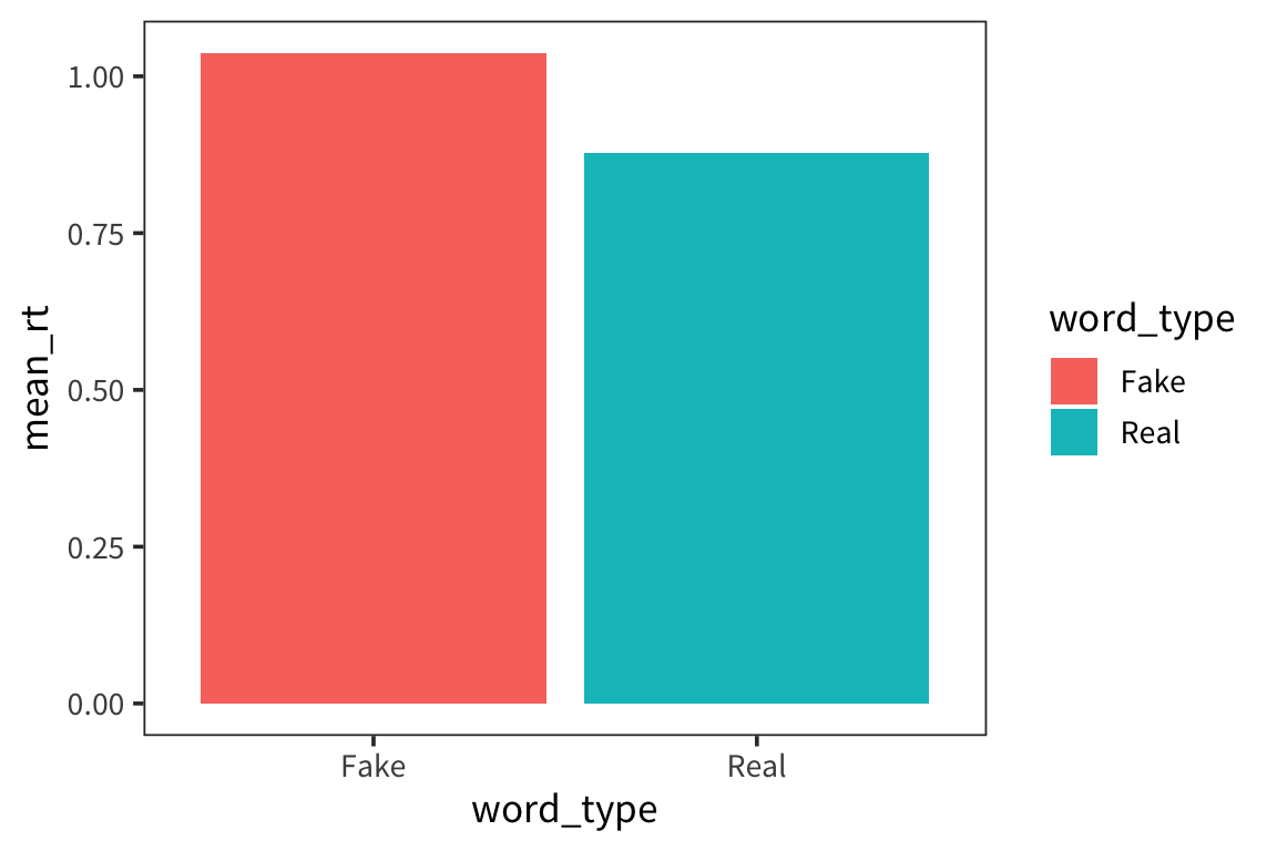

This again shows us that fake words lead to slower responses but we have no information about how variable the data are within each bar. This is one of the main problems with using bar charts. To try to get at the variability, people often use error bars (which I will show you how to add after we discuss standard error and confidence intervals).

Lab 1

Calculator

Variables

Functions

Vectors

Characters

NA

Logicals

Try it yourself…

Dataframes

Data manipulation (dplyr)

mutate

filter

select

arrange

group_by and summarise

%>%

Try it yourself…

Data visualization (ggplot2)

Histograms

Scatterplots

Facets

Boxplots

Violin plots

Barplots

Data manipulation (`dplyr`)

`mutate`

`filter`

`select`

`arrange`

`group_by` and `summarise`

`%>%`

Data visualization (`ggplot2`)