Lab 6
9.59 Lab in Psycholinguistics
data_source <- "http://web.mit.edu/psycholinglab/www/data/"
rts <- read_csv(file.path(data_source, "rts.csv"))
Lab 5 review
Take a look at the
lexdecdataset in thelanguageRpackage. Make a plot with RT plotted against Length, facetted by NativeLanguage What do you hypothesize about the relationships between these variables?Fit a model with RT as the response variable and Length as the predictor. What is the interpretation of the effect of Length on RT?
Fit a model with RT as the response variable and Length and NativeLanguage as the predictors. What is the interpretation of effects of Length and Native Language on RT?
Fit a model with RT as the response variable and Length, NativeLanguage, and their interaction as the predictors. Now what is the interpretation of effects of Length and Native Language on RT?
What is the r2 of each of these models? Which is the best fitting?
For both the model with and without the interaction term, use
augment()to get the fitted values for each combination of Length and NativeLanguage in the data.Plot these fitted values as lines, using color to indicate NativeLanguage.
library(tidyverse)
library(languageR)
library(broom)

ggplot(lexdec, aes(x = Length, y = RT)) +
  facet_wrap(vars(NativeLanguage)) +
  geom_jitter() +
  geom_smooth(method = "lm")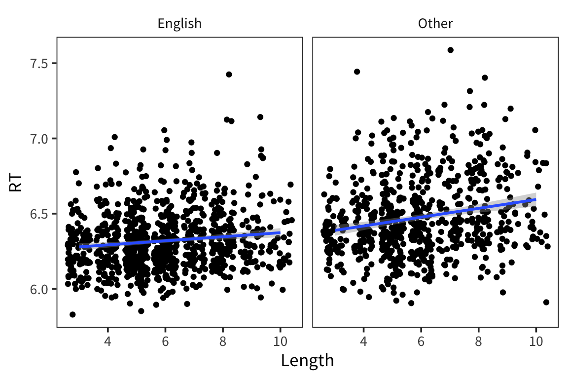
contrasts(lexdec$NativeLanguage) <- contr.sum

lexdec_length <- lm(RT ~ Length, data = lexdec)
summary(lexdec_length)
##
## Call:
## lm(formula = RT ~ Length, data = lexdec)
##
## Residuals:
## Min 1Q Median 3Q Max
## -0.5571 -0.1640 -0.0364 0.1199 1.1802
##
## Coefficients:
## Estimate Std. Error t value Pr(>|t|)
## (Intercept) 6.265354 0.019550 320.47 < 2e-16 ***
## Length 0.020255 0.003155 6.42 1.78e-10 ***
## ---
## Signif. codes: 0 '***' 0.001 '**' 0.01 '*' 0.05 '.' 0.1 ' ' 1
##
## Residual standard error: 0.2386 on 1657 degrees of freedom
## Multiple R-squared: 0.02427, Adjusted R-squared: 0.02368
## F-statistic: 41.21 on 1 and 1657 DF, p-value: 1.78e-10lexdec_length_native <- lm(RT ~ Length + NativeLanguage, data = lexdec)
summary(lexdec_length_native)##
## Call:
## lm(formula = RT ~ Length + NativeLanguage, data = lexdec)
##
## Residuals:
## Min 1Q Median 3Q Max
## -0.64615 -0.15142 -0.03568 0.11595 1.09113
##
## Coefficients:
## Estimate Std. Error t value Pr(>|t|)
## (Intercept) 6.276484 0.018523 338.846 < 2e-16 ***
## Length 0.020255 0.002987 6.782 1.65e-11 ***
## NativeLanguage1 -0.077911 0.005603 -13.905 < 2e-16 ***
## ---
## Signif. codes: 0 '***' 0.001 '**' 0.01 '*' 0.05 '.' 0.1 ' ' 1
##
## Residual standard error: 0.2259 on 1656 degrees of freedom
## Multiple R-squared: 0.1263, Adjusted R-squared: 0.1252
## F-statistic: 119.7 on 2 and 1656 DF, p-value: < 2.2e-16##
## Call:
## lm(formula = RT ~ Length * NativeLanguage, data = lexdec)
##
## Residuals:
## Min 1Q Median 3Q Max
## -0.68315 -0.15031 -0.03537 0.11609 1.08128
##
## Coefficients:
## Estimate Std. Error t value Pr(>|t|)
## (Intercept) 6.269796 0.018664 335.924 < 2e-16 ***
## Length 0.021387 0.003012 7.100 1.85e-12 ***
## NativeLanguage1 -0.031096 0.018664 -1.666 0.09589 .
## Length:NativeLanguage1 -0.007919 0.003012 -2.629 0.00864 **
## ---
## Signif. codes: 0 '***' 0.001 '**' 0.01 '*' 0.05 '.' 0.1 ' ' 1
##
## Residual standard error: 0.2255 on 1655 degrees of freedom
## Multiple R-squared: 0.1299, Adjusted R-squared: 0.1283
## F-statistic: 82.37 on 3 and 1655 DF, p-value: < 2.2e-16predictors <- lexdec %>% distinct(Length, NativeLanguage)
fits_length_native <- augment(lexdec_length_native, newdata = predictors)
fits_interaction <- augment(lexdec_interaction, newdata = predictors)
ggplot(fits_length_native,
aes(x = Length, y = .fitted, colour = NativeLanguage)) +
geom_line()
ggplot(fits_interaction,
       aes(x = Length, y = .fitted, colour = NativeLanguage)) +
  geom_line() +
  geom_line(aes(y = .fitted + 1.96 * .se.fit), linetype = "dashed") +
  geom_line(aes(y = .fitted - 1.96 * .se.fit), linetype = "dashed")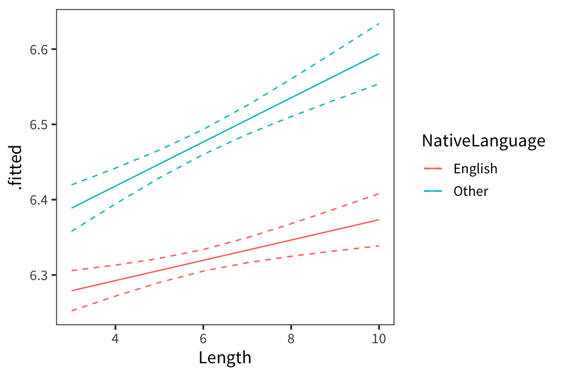
Logistic regression
So far we’ve dealt with data where the dependent variable is some continuous quantity, in this case we’ve looked at RTs. But often in linguistics we want to answer a categorical question. For example, we may want to see what predicts people’s tendency to say “yes” or “no”, as in the typical comprehension question. In cases where the possible values of the dependent variable are 0 or 1, it’s no longer appropriate to use linear regression, because linear regression produces values all over the number line.
For this part, let’s imagine that we care about slow vs. fast RTs more coarsely.
rts_binary <- rts %>%
  mutate(rt_binary = if_else(RTlexdec > 6.5, 1, 0))

ggplot(rts_binary, aes(x = WrittenFrequency, y = rt_binary)) +
  geom_point(shape = 1) +
  geom_smooth(method = "glm", method.args = list(family = "binomial"))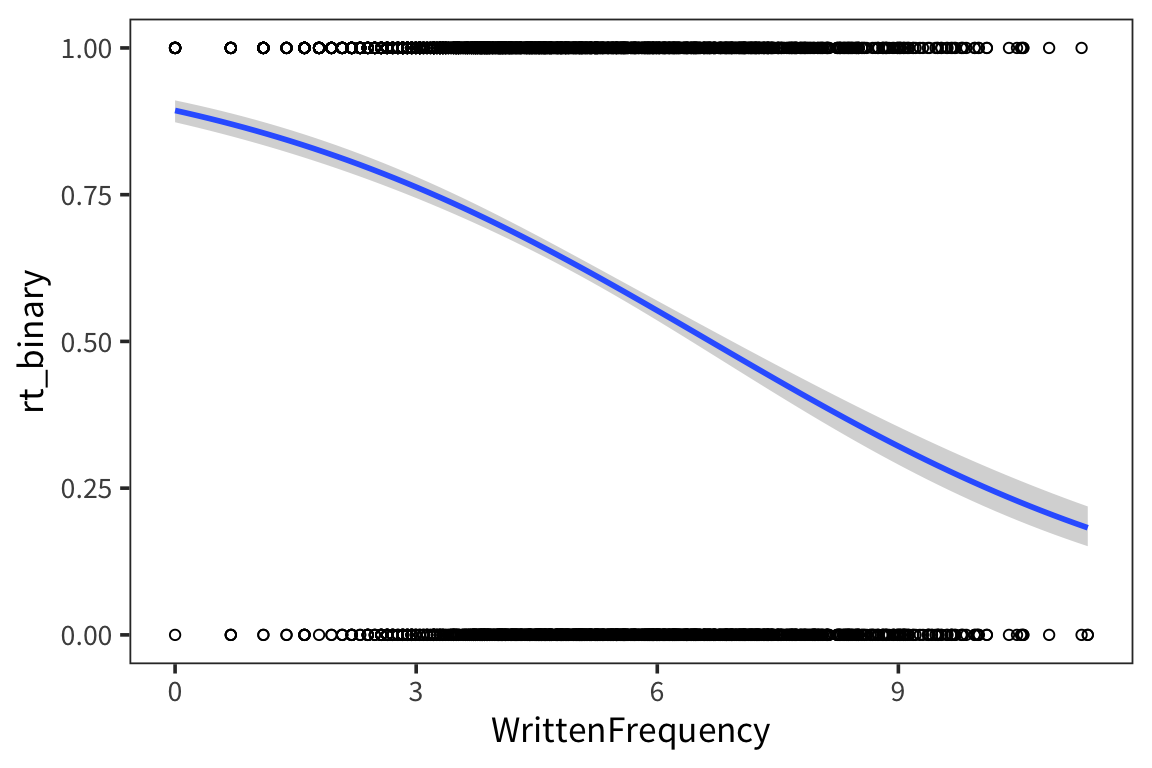
You can see that all the values are 0s and 1s so that makes it hard to see a pattern.
Let’s bin the x-axis and get means within each bin just to get an idea…
rts_binned <- rts_binary %>%
  mutate(freq_bin = cut(WrittenFrequency, 20)) %>%
  group_by(freq_bin) %>%
  summarise(mean_rt = mean(rt_binary))

ggplot(rts_binned, aes(x = freq_bin, y = mean_rt)) +
  geom_point() +
  theme(axis.text.x = element_text(angle = 45, hjust = 1, size = 8))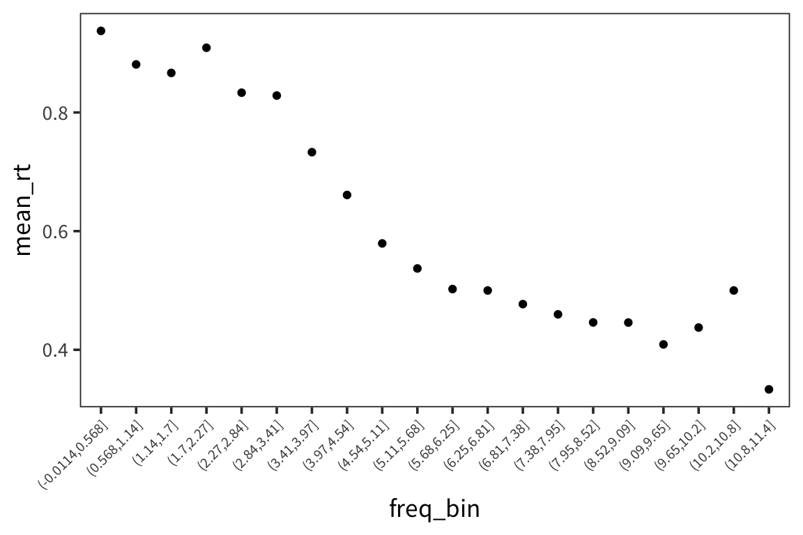
So we see a familiar relationship: the higher the written frequency, the more likely that the average RT is closer to 0.
But rt_binary is a binary variable (1 or 0) so if we want that to be our outcome, the normal distribution is not appropriate. The errors are not normally distributed around the expected values – it’s all 0s and 1s. We’re no longer interested in predicting number values, but rather in classifying our data as 0 or 1. Our generative process should be something that gets a probability that something is in class 1, then flips a coin with that probability to determine its class.
Instead of a normal distribution here, let’s use a bernoulli distribution. A bernoulli distribution takes one parameter, called \(p\), and returns 1 with probability \(p\), and 0 with probability \(1 - p\).
## [1] TRUE TRUE TRUE FALSE FALSE TRUE FALSE FALSE FALSE FALSESo we can still use the concepts from linear regression where we have an intercept \(\beta_0\) and slope \(\beta_1\) to figure out the probability of a \(y\) being 1 or 0 given a certain \(x\) and then submit that to the bernoulli distribution.
\[ p = \beta_0 + \beta_1 \cdot x_1 + \beta_2 \cdot x_2 + ... \] \[ y \sim \text{Bernoulli}(p) \]
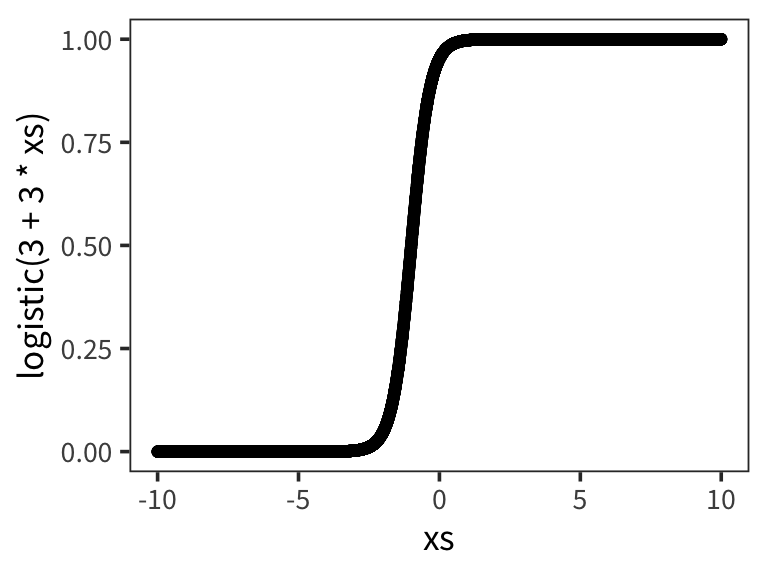
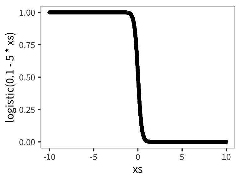
Okay, but the problem is a probability has to be between 0 and 1, and there’s no guarantee that this expression will do that. In our expression so far, p could be any real number from negative infinity to infinity. So let’s just run it through a function which takes real numbers, then squashes them into the space between 0 and 1 by generating values that are like .9999 or .97 or .0001. So we want the values coming out of our model to be really close to 1, or really close to 0, which is similar to our real data. Then if the value is less than .5 we count that as a prediction of 0 and if it’s greater than .5 we count it as a prediction of 1.
That is the logistic function. In particular it makes 0 into .5.
logistic <- function(x) {
  exp(x) / (1 + exp(x))
}

xs <- runif(10000, -10, 10)
qplot(xs, logistic(xs))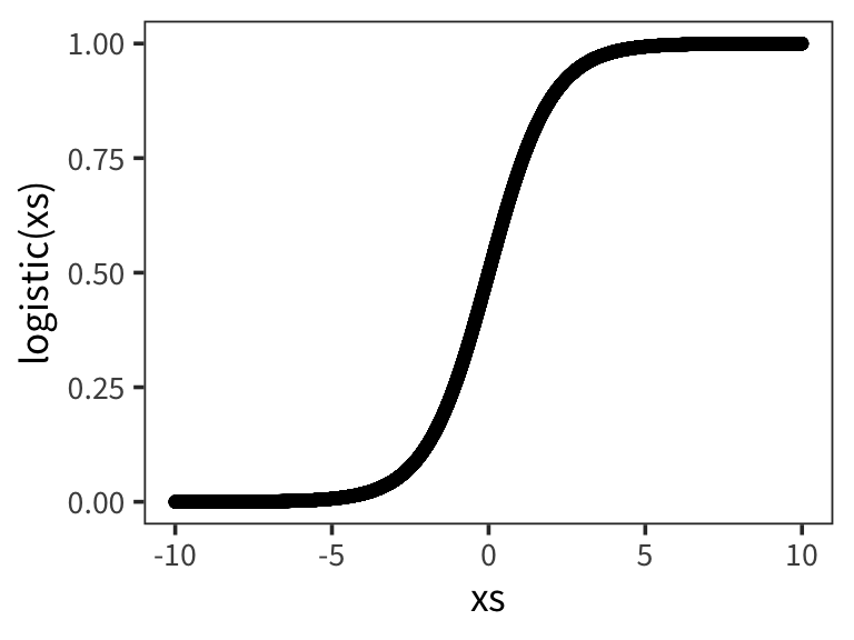
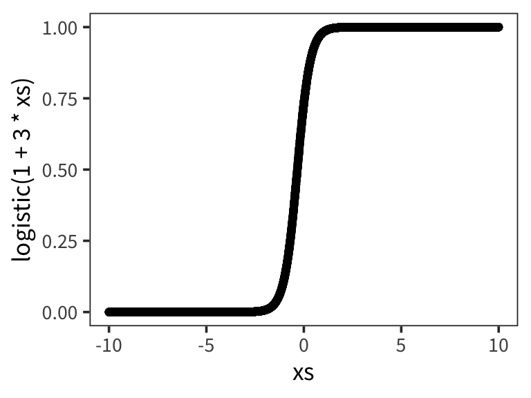
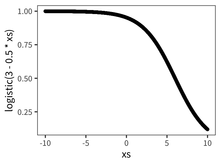
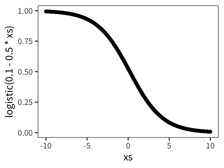
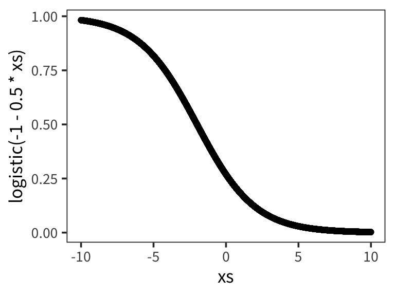
Let’s try out a few different possible \(\beta_0\) and \(\beta_1\) values to get a sense of how the logistic function changes as function of them:
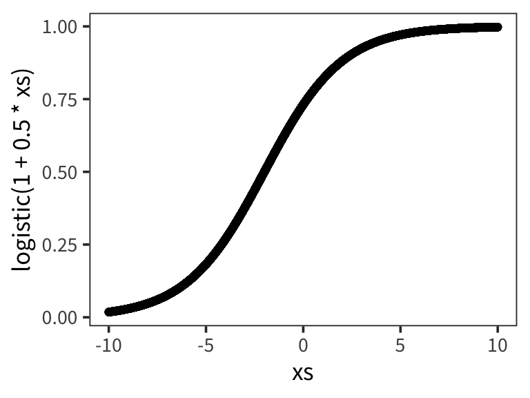
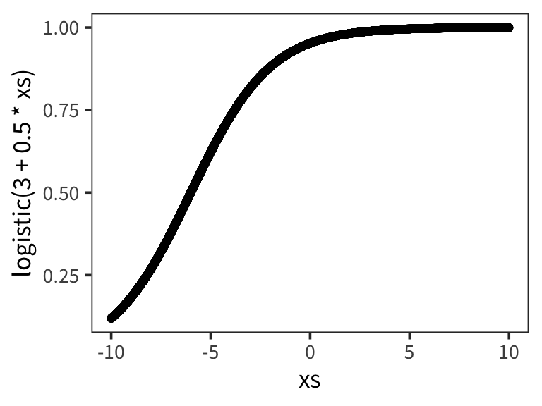
Now we’ll say:
\[ p = \text{logistic}( \beta_0 + \beta_1 \cdot x_1 + \beta_2 \cdot x_2 + ... ) \]
So let’s run a logistic regression. The syntax is very similar to linear regression:
freq_glm <- glm(rt_binary ~ WrittenFrequency, data = rts_binary,
                family = binomial(link = "logit"))
summary(freq_glm)
##
## Call:
## glm(formula = rt_binary ~ WrittenFrequency, family = binomial(link = "logit"),
## data = rts_binary)
##
## Deviance Residuals:
## Min 1Q Median 3Q Max
## -2.1163 -1.2300 0.7402 0.9421 1.8335
##
## Coefficients:
## Estimate Std. Error z value Pr(>|z|)
## (Intercept) 2.12664 0.09975 21.32 <2e-16 ***
## WrittenFrequency -0.31928 0.01813 -17.61 <2e-16 ***
## ---
## Signif. codes: 0 '***' 0.001 '**' 0.01 '*' 0.05 '.' 0.1 ' ' 1
##
## (Dispersion parameter for binomial family taken to be 1)
##
## Null deviance: 6068.0 on 4567 degrees of freedom
## Residual deviance: 5726.2 on 4566 degrees of freedom
## AIC: 5730.2
##
## Number of Fisher Scoring iterations: 4freq_glm_tidy <- tidy(freq_glm)
intercept <- filter(freq_glm_tidy, term == "(Intercept)")$estimate
slope <- filter(freq_glm_tidy, term == "WrittenFrequency")$estimate
newxs <- runif(10000, 0, 10)
freq_logistic <- logistic(intercept + slope * newxs)
qplot(newxs, freq_logistic)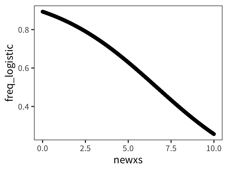
At the top we have some information about the residuals (same as with linear regression), but here they don’t need to be normally distributed.
At the very bottom there are some descriptions of how well the model is fitting the data. One test asks whether the model with predictors fits significantly better than a model with just an intercept (i.e., a null model). The test statistic is the difference between the residual deviance for the model with predictors and the null model. It is chi-square distributed with degrees of freedom equal to the differences in degrees of freedom between the current and the null model (i.e. the number of predictor variables in the model). You could compute it but it’s not super informative. AIC is similar - it’s useful for comparing models. The iteration is a measure of how much time it took to find the best estimate.
Now the coefficients are somewhat harder to interpret than in linear regression:
The intercept corresponds to the log odds of being in the slow RT group (RTbin=1) when WrittenFrequency is 0. In other words, the odds of being slow for words with frequency 0 is pretty high. In this case this is not super useful information. In general, the intercept is often less interesting in logistic regression.
Earlier, we could say that the slope corresponded the change in \(y\) for 1 unit change of \(x\). Here, it’s the same thing, but then squashed in the logistic function, so it’s a little harder to map onto some meaningful numbers.
Let’s see what happens if we pull out some plausible values of frequency.
## [1] 0.6295346## [1] 0.5525395predicted <- augment(freq_glm, newdata = data_frame(WrittenFrequency = c(5, 6)),
type.predict = "response")So the probability of a slow RT, when Frequency is 5, is 0.63 and the probability of a slow RT is 0.55 for Frequency = 6. Now we can reconstruct the slope by looking at a 1 unit increase in Frequency by taking the difference of the log odds.
log_odds_5 <- log(predicted$.fitted[1] / (1 - predicted$.fitted[1]))
log_odds_6 <- log(predicted$.fitted[2] / (1 - predicted$.fitted[2]))

diff_log_odds <- log_odds_6 - log_odds_5
diff_log_odds
## [1] -0.3192841You can still take a larger slope to indicate a larger effect, but now instead of 1 unit change in \(x\) being equal to 1 unit change in \(y\), it means 1 unit change in WrittenFrequency corresponds to a -0.32 change in log odds of RTbin being 1, i.e. of a slow reaction time.
It’s pretty hard to imagine what it means for something to decrease in log-odds space. By exponentiating we can think about the odds ratio (odds for \(x=6\) / odds for \(x=5\)).
## [1] 0.7266691This says that the odds of RT being categorized as slow are multiplied by 0.73 (i.e. < 1 means decreases) with every additional unit of WrittenFrquency.
Because the relationship between \(p(x)\) and \(x\) is not linear, we can’t easily say anything about the change in proportions for a unit change in \(x\).
What about categorical predictors?
rts_binary <- rts_binary %>%
  mutate(AgeSubject = factor(AgeSubject))

age_glm <- glm(rt_binary ~ AgeSubject, data = rts_binary,
               family = binomial(link = "logit"))
summary(age_glm)
##
## Call:
## glm(formula = rt_binary ~ AgeSubject, family = binomial(link = "logit"),
## data = rts_binary)
##
## Deviance Residuals:
## Min 1Q Median 3Q Max
## -2.6242 -0.7959 0.2549 0.2549 1.6149
##
## Coefficients:
## Estimate Std. Error z value Pr(>|z|)
## (Intercept) 3.4107 0.1190 28.67 <2e-16 ***
## AgeSubjectyoung -4.3980 0.1279 -34.38 <2e-16 ***
## ---
## Signif. codes: 0 '***' 0.001 '**' 0.01 '*' 0.05 '.' 0.1 ' ' 1
##
## (Dispersion parameter for binomial family taken to be 1)
##
## Null deviance: 6068.0 on 4567 degrees of freedom
## Residual deviance: 3317.3 on 4566 degrees of freedom
## AIC: 3321.3
##
## Number of Fisher Scoring iterations: 6ggplot(rts_binary, aes(x = WrittenFrequency, y = rt_binary, colour = AgeSubject)) +
geom_point(shape = 1) +
geom_smooth(method = "glm", method.args = list(family = "binomial"))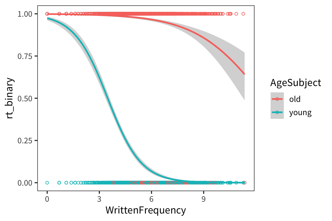
Try it yourself…
Use the coefficients from the age model to recover the predicted probabilities of being slow for old subjects and for being slow for young subjects.
Recover the slope from these two probabilities.
age_glm_tidy <- tidy(age_glm)

intercept <- filter(age_glm_tidy, term == "(Intercept)")$estimate
slope <- filter(age_glm_tidy, term == "AgeSubjectyoung")$estimate

old_code <- contrasts(rts_binary$AgeSubject)["old", ]
young_code <- contrasts(rts_binary$AgeSubject)["young", ]

# probability of slow given old
old <- logistic(intercept + slope * old_code)

# probability of slow given young
young <- logistic(intercept + slope * young_code)

(young / (1 - young)) / (old / (1 - old))
## [1] 0.01230191## [1] 0.01230191
Mixed-effects models
One important assumption of all these models is that we have been pretending that all the data points in our scatter plot are generated independently from calls to some generative process like rnorm. But that’s not how experiments usually work…
Usually each subject sees a bunch of items in one of several conditions. And the same items are seen by many subjects (sometimes there are different lists but sometimes all subjects see all items).
There will be some correlation between datapoints within subjects, because maybe some subjects are sleepy and tend to respond slowly, or others just drank a bunch of coffee and are responding super fast. This correlation is entirely missed in our regression model here. We’re analyzing our data as if it was between-subjects, and consequently we’re losing statistical power. Same thing with the items. We know now that words have properties that affect how people respond to them so subjects’ responses will be correlated for a the same items.
Let’s look at this in the lexdec dataset:
lexdec_subject <- lexdec %>%
  group_by(Subject) %>%
  summarise(mean_rt = mean(RT))

ggplot(lexdec, aes(x = Subject, y = RT)) +
  geom_point(shape = 1, colour = "grey") +
  geom_point(aes(y = mean_rt), data = lexdec_subject, size = 3)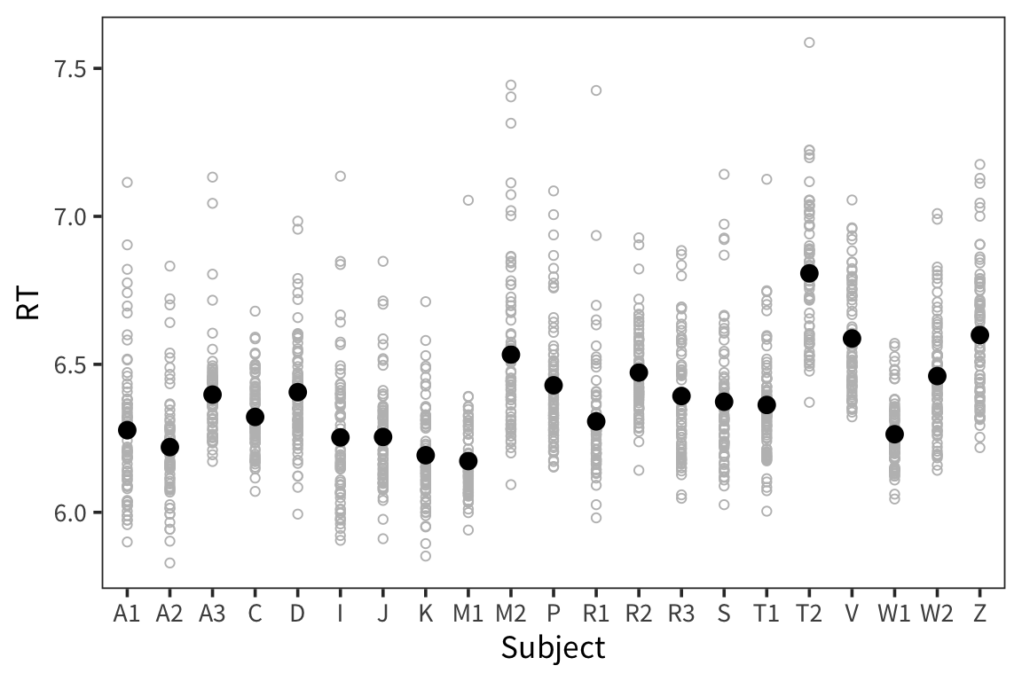
You can see that the different subjects have different average RTs and they also vary in terms of how they are affected by the the predictor of interest:
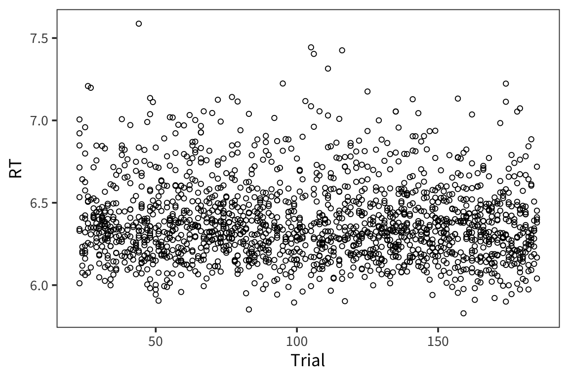
ggplot(lexdec, aes(x = Trial, y = RT)) +
  facet_wrap(~Subject) +
  geom_point(shape = 1) +
  geom_smooth(method = "lm")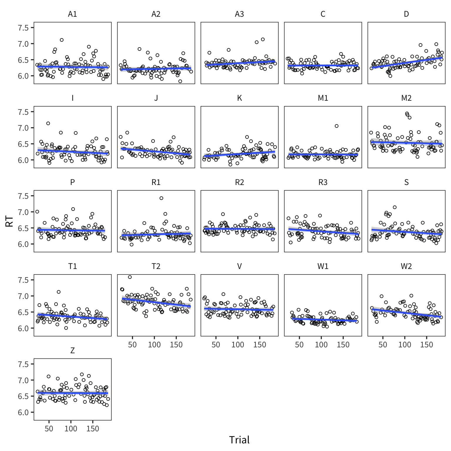
Same thing if we look at items:
lexdec_items <- lexdec %>%
  group_by(Word) %>%
  summarise(mean_rt = mean(RT))

ggplot(lexdec_items, aes(x = Word, y = mean_rt)) +
  geom_text(aes(label = Word)) +
  theme(axis.text.x = element_text(angle = 45, hjust = 1, size = 8))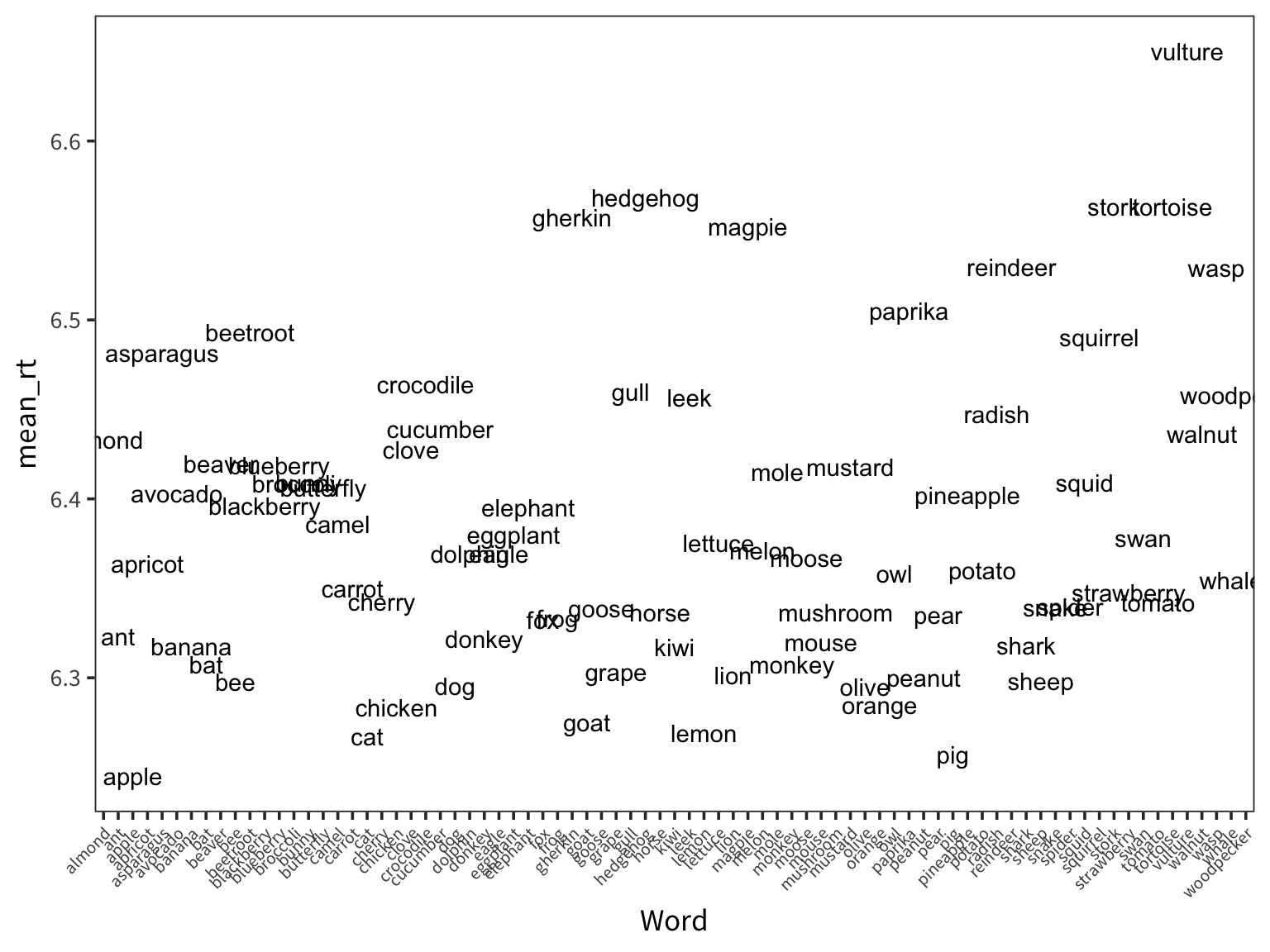
ggplot(lexdec, aes(x = Trial, y = RT)) +
  facet_wrap(~Word) +
  geom_point(shape = 1) +
  geom_smooth(method = "lm")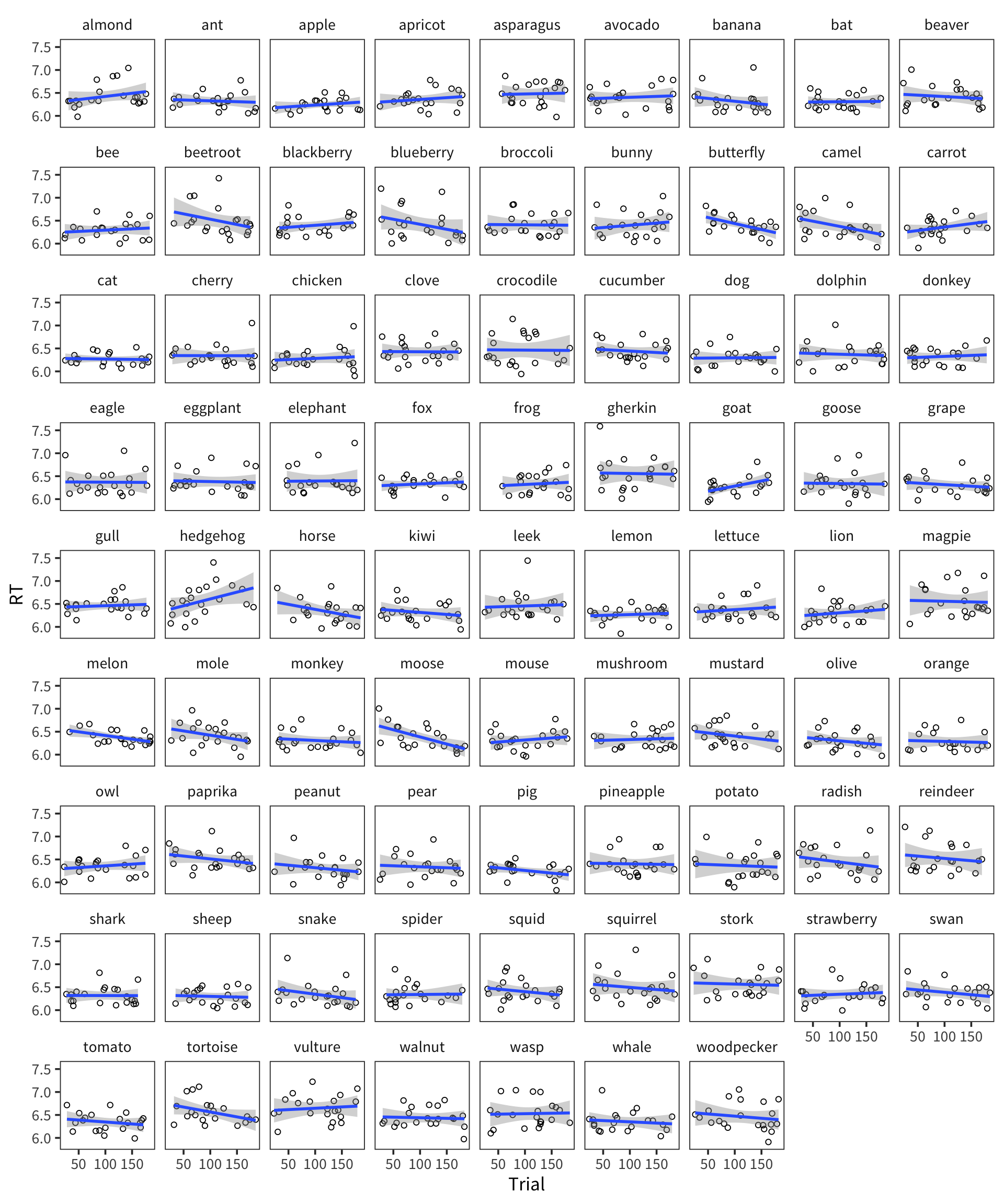
We’re going to have to change our generative process for our data, such that the generative process generates datapoints that are correlated within subject and within item.
##
## Call:
## lm(formula = RT ~ Trial, data = lexdec)
##
## Residuals:
##      Min       1Q   Median       3Q      Max
## -0.53961 -0.16943 -0.04366  0.11594  1.18357
##
## Coefficients:
##               Estimate Std. Error t value Pr(>|t|)
## (Intercept)  6.4172041  0.0144549 443.948   <2e-16 ***
## Trial       -0.0003060  0.0001256  -2.435    0.015 *
## ---
## Signif. codes:  0 '***' 0.001 '**' 0.01 '*' 0.05 '.' 0.1 ' ' 1
##
## Residual standard error: 0.2412 on 1657 degrees of freedom
## Multiple R-squared:  0.003567,   Adjusted R-squared:  0.002965
## F-statistic: 5.931 on 1 and 1657 DF,  p-value: 0.01498
Previously we had: \[ y_i \sim \mathcal{N}(\mu_i, \sigma) \] \[ \mu_i = \beta_0 + \beta_1 \cdot x_{1_i} + \beta_2 \cdot x_{2_i} + \beta_3 \cdot x_{1_i} \cdot x_{2_i} \]
Now let’s incorporate the fact that each subject and each item has its own mean.
\[ y_i \sim \mathcal{N}(\mu_i, \sigma) \] \[ \mu_i = \beta_0 + \gamma_{s_i} + \gamma_{j_i} + ... \]
So the intercept for a particular datapoint will not just be \(\beta_0\), but rather \(\beta_0\) plus \(\gamma_s\) for the particular subject, plus \(\gamma_j\) for the particular item. So now we have incorporated different intercepts for different subjects and items in our model. We need to take one more step.
In general, while we know there is variation between subjects and items, we don’t think that variation is without bound. We think most subject means will be around the same, and most item means will be around the same.
So instead of just having these numbers here, let’s draw these numbers from a normal distribution:
\[ y_i \sim \mathcal{N}(\mu_i, \sigma) \] \[ \mu_i = \beta_0 + \gamma_{s_i} + \gamma_{j_i} + ... \] \[ \gamma_{s_i} \sim \mathcal{N}(0, \sigma_s) \] \[ \gamma_{j_i} \sim \mathcal{N}(0, \sigma_j) \]
This says the value of \(\gamma_{s_i}\) is probably 0, and with some probability as determined by the normal distribution it is some other value with some distance from 0.
\(\gamma_{s_i}\) is the extent to which the intercept for subject will differ from the mean intercept of all subjects.
Then we generate a \(\gamma_{j_i}\) for an item. Then we generate our data from a normal distribution around that mean.
Random intercepts
library(lme4)
library(lmerTest)
library(broom.mixed)

subject_lmer <- lmer(RT ~ Trial + (1 | Subject), data = lexdec)
summary(subject_lmer)
## Linear mixed model fit by REML. t-tests use Satterthwaite's method [
## lmerModLmerTest]
## Formula: RT ~ Trial + (1 | Subject)
## Data: lexdec
##
## REML criterion at convergence: -720.2
##
## Scaled residuals:
## Min 1Q Median 3Q Max
## -2.2919 -0.6592 -0.1547 0.4585 5.9198
##
## Random effects:
## Groups Name Variance Std.Dev.
## Subject (Intercept) 0.02362 0.1537
## Residual 0.03565 0.1888
## Number of obs: 1659, groups: Subject, 21
##
## Fixed effects:
## Estimate Std. Error df t value Pr(>|t|)
## (Intercept) 6.410e+00 3.540e-02 2.391e+01 181.06 <2e-16 ***
## Trial -2.348e-04 9.866e-05 1.637e+03 -2.38 0.0174 *
## ---
## Signif. codes: 0 '***' 0.001 '**' 0.01 '*' 0.05 '.' 0.1 ' ' 1
##
## Correlation of Fixed Effects:
## (Intr)
## Trial -0.292subject_item_lmer <- lmer(RT ~ Trial + (1 | Subject) + (1 | Word), data = lexdec)
summary(subject_item_lmer)## Linear mixed model fit by REML. t-tests use Satterthwaite's method [
## lmerModLmerTest]
## Formula: RT ~ Trial + (1 | Subject) + (1 | Word)
## Data: lexdec
##
## REML criterion at convergence: -889.2
##
## Scaled residuals:
## Min 1Q Median 3Q Max
## -2.2877 -0.6281 -0.1255 0.4695 5.9639
##
## Random effects:
## Groups Name Variance Std.Dev.
## Word (Intercept) 0.005917 0.07692
## Subject (Intercept) 0.023688 0.15391
## Residual 0.029727 0.17242
## Number of obs: 1659, groups: Word, 79; Subject, 21
##
## Fixed effects:
## Estimate Std. Error df t value Pr(>|t|)
## (Intercept) 6.410e+00 3.623e-02 2.621e+01 176.917 <2e-16 ***
## Trial -2.421e-04 9.144e-05 1.580e+03 -2.647 0.0082 **
## ---
## Signif. codes: 0 '***' 0.001 '**' 0.01 '*' 0.05 '.' 0.1 ' ' 1
##
## Correlation of Fixed Effects:
## (Intr)
## Trial -0.265So in addition to the fixed effects you see random effects! Fixed effects are the things we care about / that we are testing, generally.
## # A tibble: 2 x 1
##   `ranef(subject_item_lmer)`
##   <named list>
## 1 <df[,1] [79 × 1]>
## 2 <df[,1] [21 × 1]>
lmer_augmented <- augment(subject_item_lmer)
ggplot(lmer_augmented, aes(x = Trial)) +
geom_point(aes(y = .fitted, colour = Subject), shape = 1) +
geom_point(aes(y = .fixed), colour = "red")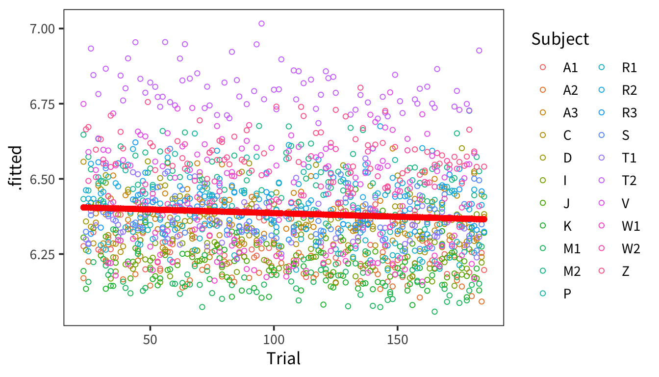
ggplot(lmer_augmented, aes(x = Trial)) +
  facet_wrap(~Subject) +
  geom_point(aes(y = .fitted, colour = Subject), shape = 1) +
  geom_point(aes(y = .fixed), colour = "red")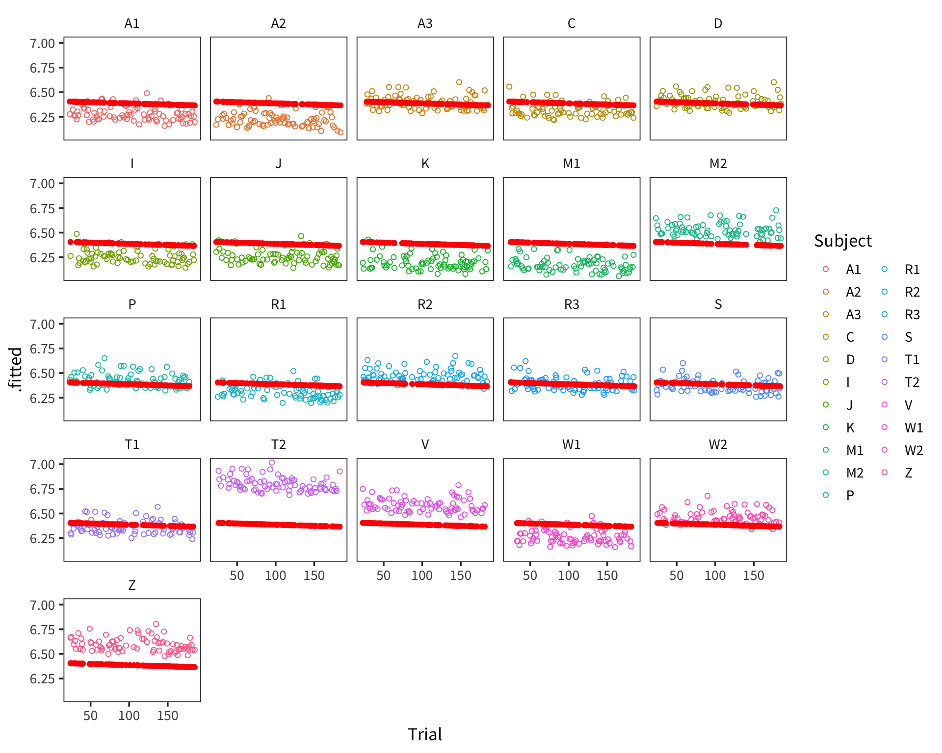
This kind of model is called a mixed effects regression with random intercepts. Our old coefficients here are called fixed effects because they are fixed in value across all datapoints. Our new coefficients \(\gamma\) are called random effects because they are drawn for each subject and item randomly from a normal distribution.
Random slopes
But you may find that not only do subjects and items have baseline differences, they may also be differentially affected by your experimental manipulation.
ggplot(lexdec, aes(x = Trial, y = RT)) +
  geom_smooth(aes(colour = Word), method = "lm", se = FALSE, size = 0.5) +
  geom_smooth(method = "lm", se = FALSE, color = "black") +
  scale_color_discrete(guide = FALSE)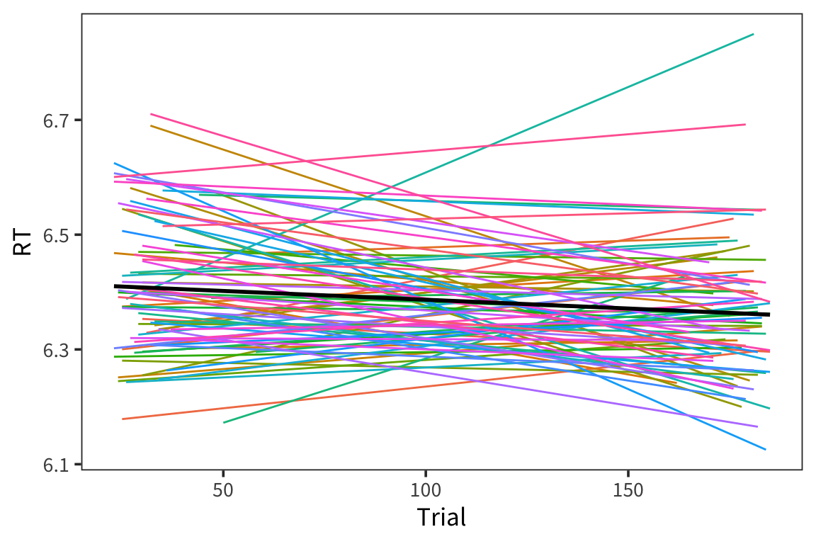
ggplot(lexdec, aes(x = Trial, y = RT)) +
  geom_smooth(aes(colour = Subject), method = "lm", se = FALSE, size = 0.5) +
  geom_smooth(method = "lm", se = FALSE, color = "black") +
  scale_color_discrete(guide = FALSE)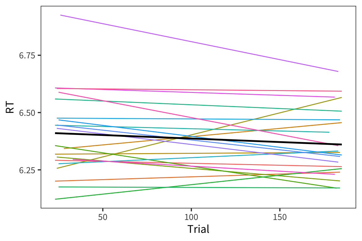
In these cases you can run mixed effects regression with random slopes. Here is the syntax for adding slopes:
Sometimes lmer will fail to find a good set of parameter values for you. The first things to try in these cases is to double-check that your model formula is correct and then to scale any continuous predictors.
lexdec_scaled <- lexdec %>%
  mutate(Trial = as.numeric(scale(Trial)))

slopes_lmer <- lmer(RT ~ Trial + (Trial | Subject) + (Trial | Word),
                    data = lexdec_scaled)
summary(slopes_lmer)
## Linear mixed model fit by REML. t-tests use Satterthwaite's method [
## lmerModLmerTest]
## Formula: RT ~ Trial + (Trial | Subject) + (Trial | Word)
## Data: lexdec_scaled
##
## REML criterion at convergence: -927
##
## Scaled residuals:
## Min 1Q Median 3Q Max
## -2.3633 -0.6100 -0.0973 0.4655 6.0248
##
## Random effects:
## Groups Name Variance Std.Dev. Corr
## Word (Intercept) 5.946e-03 0.077110
## Trial 2.068e-06 0.001438 -1.00
## Subject (Intercept) 2.366e-02 0.153828
## Trial 1.093e-03 0.033068 -0.31
## Residual 2.869e-02 0.169377
## Number of obs: 1659, groups: Word, 79; Subject, 21
##
## Fixed effects:
## Estimate Std. Error df t value Pr(>|t|)
## (Intercept) 6.385124 0.034921 22.678019 182.847 <2e-16 ***
## Trial -0.011505 0.008374 19.767896 -1.374 0.185
## ---
## Signif. codes: 0 '***' 0.001 '**' 0.01 '*' 0.05 '.' 0.1 ' ' 1
##
## Correlation of Fixed Effects:
## (Intr)
## Trial -0.259
## convergence code: 0
## boundary (singular) fit: see ?isSingularThere are also some other tricks to try. If you can’t get it converge, it often means that you do not have enough data to fit all the parameters you are looking for. This is not great but there’s a semi-reasonable (or at least this is currently the best approach we’ve got) way to deal with it. You take out terms from the random effects structure in stepwise fashion until the model converges.
You can also model binary variables with mixed-effects models using glmer() and the family="binomial" argument.
Great visualization of mixed effects modeling: http://mfviz.com/hierarchical-models/
More information on glmm models: http://bbolker.github.io/mixedmodels-misc/glmmFAQ.html#model-specification
Try it yourself…
- Using the
lexdecdataset from the beginning of the lab, fit the mixed effects version of the same model. Include a random intercept for Word, a random intercept for Subject, and a random slope of Length for Subject. - Compare the results from the mixed effects model to the original model. What stayed the same? What changed?
- Pick a word and a subject and recover the predicted RT for that subject on that word from the model.
- Compare this fitted value to the result from
augment(). - Plot the fitted line for each subject.
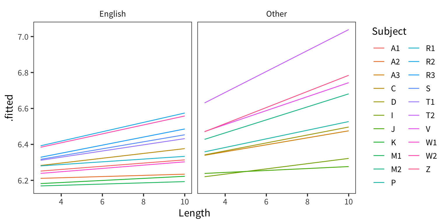
- Use
augment()with thenewdataargument to generate fits for each combination of Subject, NativeLanguage, and Length. (Hint: the argumentre.formlet’s you specify which random effects to include. Ignore any warnings.) - Plot the fitted RT against Length, facetted by NativeLanguage, with a colour for each subject.
- Use
lexdec_mm <- lmer(RT ~ Length * NativeLanguage + (Length | Subject) + (1 | Word),
                  data = lexdec)

tidy(lexdec_mm) %>% filter(effect == "fixed")
## # A tibble: 4 x 8
## effect group term estimate std.error statistic df p.value
## <chr> <chr> <chr> <dbl> <dbl> <dbl> <dbl> <dbl>
## 1 fixed <NA> (Intercept) 6.27 0.0330 190. 60.7 5.85e-86
## 2 fixed <NA> Length 0.0214 0.00554 3.86 57.6 2.91e- 4
## 3 fixed <NA> NativeLanguage1 -0.0311 0.0210 -1.48 19.0 1.56e- 1
## 4 fixed <NA> Length:NativeLa… -0.00792 0.00373 -2.13 19.0 4.69e- 2## # A tibble: 4 x 5
## term estimate std.error statistic p.value
## <chr> <dbl> <dbl> <dbl> <dbl>
## 1 (Intercept) 6.27 0.0187 336. 0.
## 2 Length 0.0214 0.00301 7.10 1.85e-12
## 3 NativeLanguage1 -0.0311 0.0187 -1.67 9.59e- 2
## 4 Length:NativeLanguage1 -0.00792 0.00301 -2.63 8.64e- 3word <- "dog"
subject <- "A1"
effects <- fixef(lexdec_mm)
ranef_subject <- ranef(lexdec_mm)$Subject[subject,]
ranef_word <- ranef(lexdec_mm)$Word[word,]
intercept <- effects[["(Intercept)"]] + ranef_subject[["(Intercept)"]] +
ranef_word
slope_length <- effects[["Length"]] + ranef_subject[["Length"]]
slope_native <- effects[["NativeLanguage1"]]
interaction <- effects[["Length:NativeLanguage1"]]
word_length <- 3
subject_langauge <- lexdec %>% filter(Subject == subject) %>%
distinct(NativeLanguage)
english_code <- contrasts(lexdec$NativeLanguage)["English",]
intercept + slope_length * word_length + slope_native * english_code +
interaction * word_length * english_code## English
## 6.228147## [1] 6.228147lexdec_subject <- lexdec %>% distinct(Subject, NativeLanguage, Length)
subject_fits <- augment(lexdec_mm, newdata = lexdec_subject,
re.form = ~(1 + Length | Subject))
ggplot(subject_fits, aes(x = Length, y = .fitted, colour = Subject)) +
facet_wrap(vars(NativeLanguage)) +
geom_line()