Problem set 4 solutions

In this assignment, you will analyze data from an experiment that was run on Amazon Mechanical Turk. In this experiment we tested how and whether the placement of a verb particle (i.e. the position of a particle preposition relative to a verb, for verbs like “put up”, “throw out”, …) depends on the length (in number of words) of the direct object of the verb. We show participants four kinds of sentences, in which the particle either comes early or late, and the direct object is either long or short. This is called a 2x2 design. The independent variables are: Particle position (early or late), and object length (long or short).

Example Sentences:

Joe threw the documents out. (late-short)
Joe threw the very important documents that he brought home out. (late-long)
Joe threw out the documents. (early-short)
Joe threw out the very important documents that he brought home. (early-long)

Load particle_data.csv into R. Exclude all participants from the analysis a) whose home country is not USA (Answer.country), b) whose native language is not English (Answer.English), and c) who did not answer at least 90% of the item comprehension questions correctly (Correct). Also, throw out any individual data points (not the whole participants!) that have NA for Answer.Rating. Report the number of remaining rows in the data frame after excluding these participants and data points.

particle <- read_csv("particle_shift_data.csv")

particle <- particle %>%
  select(Item, Condition, Answer.country, Answer.English, Answer.Rating,
         Participant, list, CorrectAnswer1, Correct)

particle <- particle %>%
  filter(Answer.country == "USA" & Answer.English == "yes")

particle <- particle %>%
  group_by(Participant) %>%
  mutate(accuracy = mean(Correct)) %>%
  filter(accuracy >= .9)

particle <- particle %>%
  filter(!is.na(Answer.Rating))

nrow(particle)

886

The column Condition simultaneously encodes the two independent variables. It would be better to have one independent variable per column. Use separate() to split the column Condition into two columns based on the position of the - character.
```
particle <- particle %>%
  separate(Condition, into = c("Position", "Length"), sep = "-")
```

Transform the grammaticality ratings (Answer.Rating) into z-scores with means and standard deviations estimated within subjects.

particle_z <- particle %>%
  group_by(Participant) %>%
  mutate(rating_z = (Answer.Rating - mean(Answer.Rating)) / sd(Answer.Rating))

Make a plot with the means for each condition and their 95% confidence intervals. Map one independent variable to the x axis and a color, and split the data by the other independent variable using facet_wrap(). What visual impression do you get from this plot about the differences among the conditions in this experiment?

particle_summary <- particle_z %>%
  group_by(Position, Length) %>%
  summarise(mean_rating = mean(rating_z),
            se_rating = sd(rating_z) / sqrt(n()))

ggplot(particle_summary, aes(x = Position, y = mean_rating, colour = Position)) +
  facet_wrap(~Length) +
  geom_pointrange(aes(ymin = mean_rating - 1.96 * se_rating,
                      ymax = mean_rating + 1.96 * se_rating)) +
  scale_colour_discrete(guide = FALSE)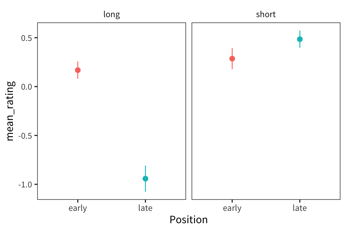

Define two dummy-coded predictors based on the independent variables (early vs. late, long vs. short). If you fit a linear regression with these predictors and their interaction, what will the coefficient of the intercept fit? What will each variable’s coefficient fit? What will the interaction term coefficient fit?
```
particle_z <- particle_z %>%
  mutate(Position = factor(Position),
         Length = factor(Length))
```
The coefficient of the intercept will fit the mean judgment for early-long items. The coefficient of Position will fit the difference between the mean judgment for late-long items and early-long items. The coefficient of Length will fit the difference between the mean judgement for early-short and early-long items. The coefficient of the interaction between Position and Length will fit the difference between the difference for late items (difference between late-short and late-long) and the difference for early items (difference between early-short and early-long).

Fit a linear regression (using lm()) to the data predicting z-scored judgments from the dummy coded predictors based on the independent variables and their interaction. Use the summary function to get the model output. Briefly describe the result.

particle_model <- lm(rating_z ~ Position * Length, data = particle_z)
summary(particle_model)

## 
## Call:
## lm(formula = rating_z ~ Position * Length, data = particle_z)
## 
## Residuals:
## 
## ------------------------------------------
##   Min       1Q      Median    3Q     Max  
## -------- --------- -------- ------ -------
##  -3.965   -0.4311   0.192    0.47   2.056 
## ------------------------------------------
## 
## 
## Coefficients:
##                          Estimate Std. Error t value Pr(>|t|)    
## (Intercept)               0.16812    0.05437   3.092  0.00205 ** 
## Positionlate             -1.11036    0.07689 -14.440  < 2e-16 ***
## Lengthshort               0.11785    0.07681   1.534  0.12528    
## Positionlate:Lengthshort  1.30904    0.10862  12.051  < 2e-16 ***
## ---
## Signif. codes:  0 '***' 0.001 '**' 0.01 '*' 0.05 '.' 0.1 ' ' 1
## 
## Residual standard error: 0.8083 on 882 degrees of freedom
## Multiple R-squared:  0.3213, Adjusted R-squared:  0.319 
## F-statistic: 139.2 on 3 and 882 DF,  p-value: < 2.2e-16

Compare the coefficient fits in the model to the predictions about them that you made in question 5 to verify that you’re interpreting the model correctly.

library(broom)
coefs <- tidy(particle_model)

cell_means <- particle_z %>%
  group_by(Position, Length) %>%
  summarise(mean = mean(rating_z))

Intercept

coefs %>% filter(term == "(Intercept)") %>% pull(estimate)

0.1681

cell_means %>% filter(Position == "early", Length == "long") %>% pull(mean)

0.1681

Position coefficient

coefs %>% filter(term == "Positionlate") %>% pull(estimate)

-1.11

filter(cell_means, Position == "late", Length == "long")$mean -
  filter(cell_means, Position == "early", Length == "long")$mean

-1.11

Length coefficient

coefs %>% filter(term == "Lengthshort") %>% pull(estimate)

0.1179

filter(cell_means, Position == "early", Length == "short")$mean -
  filter(cell_means, Position == "early", Length == "long")$mean

0.1179

Position x Length interaction coefficient

coefs %>% filter(term == "Positionlate:Lengthshort") %>% pull(estimate)

1.309

late_diff <- filter(cell_means, Position == "late", Length == "short")$mean -
  filter(cell_means, Position == "late", Length == "long")$mean
early_diff <- filter(cell_means, Position == "early", Length == "short")$mean -
  filter(cell_means, Position == "early", Length == "long")$mean
late_diff - early_diff

1.309

Extra Credit: Change the indepepent variable predictors to be effects coded rather than dummy coded. Fit the same model as before to this dataset and briefly describe the result. Do any terms change from being significant to being non-significant, or vice versa?

particle_effects <- particle_z
contrasts(particle_effects$Position) <- contr.sum
contrasts(particle_effects$Length) <- contr.sum

particle_model_effects <- lm(rating_z ~ Position * Length, data = particle_effects)
summary(particle_model_effects)

## 
## Call:
## lm(formula = rating_z ~ Position * Length, data = particle_effects)
## 
## Residuals:
## 
## ------------------------------------------
##   Min       1Q      Median    3Q     Max  
## -------- --------- -------- ------ -------
##  -3.965   -0.4311   0.192    0.47   2.056 
## ------------------------------------------
## 
## 
## Coefficients:
##                     Estimate Std. Error t value Pr(>|t|)    
## (Intercept)       -0.0008718  0.0271553  -0.032    0.974    
## Position1          0.2279185  0.0271553   8.393   <2e-16 ***
## Length1           -0.3861870  0.0271553 -14.221   <2e-16 ***
## Position1:Length1  0.3272600  0.0271553  12.051   <2e-16 ***
## ---
## Signif. codes:  0 '***' 0.001 '**' 0.01 '*' 0.05 '.' 0.1 ' ' 1
## 
## Residual standard error: 0.8083 on 882 degrees of freedom
## Multiple R-squared:  0.3213, Adjusted R-squared:  0.319 
## F-statistic: 139.2 on 3 and 882 DF,  p-value: < 2.2e-16

The Length variable is now significant.

Extra Credit: In this new model, what does each of terms (intercept, slopes, interaction) fit? Compare each term to the correponding quantities in the data to verify your interpretation.
```
coefs_effects <- tidy(particle_model_effects)
```
Intercept
```
coefs_effects %>% filter(term == "(Intercept)") %>% pull(estimate)
```
-0.0008718
```
mean(cell_means$mean)
```
-0.0008718
Position coefficient
```
coefs_effects %>% filter(term == "Position1") %>% pull(estimate)
```
0.2279
```
early <- cell_means %>% filter(Position == "early")
mean(early$mean) - mean(cell_means$mean)
```
0.2279
Length coefficient
```
coefs_effects %>% filter(term == "Length1") %>% pull(estimate)
```
-0.3862
```
long <- cell_means %>% filter(Length == "long")
mean(long$mean) - mean(cell_means$mean)
```
-0.3862
Position x Length interaction coefficient
```
coefs_effects %>% filter(term == "Position1:Length1") %>% pull(estimate)
```
0.3273
```
mean_early_long <- filter(cell_means, Position == "early", Length == "long")$mean
mean_late_short <- filter(cell_means, Position == "late", Length == "short")$mean
(mean_early_long + mean_late_short) / 2 - mean(cell_means$mean)
```
0.3273

The coefficient of the intercept fits the grand mean judgment (mean of the means of each condition). The coefficient of Position fits the difference between the mean judgment for early items and the grand mean. The coefficient of Length fits the difference between the mean judgement for long items and the grand mean. The coefficient of the interaction between Position and Length fits the mean of the means for early-long items and for late-short items, minus the grand mean.
Use the coefficients from the model (either of the two you’ve fit) to calculate the predicted group means for the four cells of the design. How far off are they from the actual group means?
```
length_codes <- contrasts(particle_effects$Length)
lengths <- tibble(Length = rownames(length_codes),
                  length_code = length_codes[,1])

position_codes <- contrasts(particle_effects$Position)
positions <- tibble(Position = rownames(position_codes),
                    position_code = position_codes[,1])

predictors <- tribble(
  ~Position, ~Length,
  "early", "short",
  "early", "long",
  "late", "short",
  "late", "long"
) %>% left_join(lengths) %>% left_join(positions)

effects <- coef(particle_model_effects)
predicted_means <- predictors %>%
  mutate(predicted = effects["(Intercept)"] +
           effects["Position1"] * position_code +
           effects["Length1"] * length_code +
           effects["Position1:Length1"] * position_code * length_code)
predicted_means %>% left_join(cell_means)
```
Using the analyses you’ve done, write a few sentences summarizing the results of the experiment.