Lab 2
Lab 1 review
Last week we started learning how to manipulate and visualize data. Let’s re-explore the in lab lexical decision task from last week.
Try it yourself…
How does RT depend on word length? Is this relationship different for real and fake words?
Plot each word’s mean RT against its length, separated by real/fake, with an lm smoother:
Load tidyverse and read in data with read_csv().
Add columns for word_type and word_length.
Get mean RT for each word.
Plot!
library(tidyverse)

rt_data <- read_csv("http://web.mit.edu/psycholinglab/www/data/in_lab_rts_2020.csv")

words <- unique(rt_data$word)
real_words <- words[c(1, 3, 5, 7, 8, 10, 12, 15, 17, 18, 21, 22)]
rt_words <- rt_data %>%
  mutate(word_length = str_length(word),
         word_type = if_else(word %in% real_words,
                             "Real", "Fake")) %>%
  group_by(word, word_type, word_length) %>%
  summarise(word_rt = mean(rt)) %>%
  ungroup() %>%
  mutate(word_type = fct_relevel(word_type,
                                 "Real", "Fake"))

ggplot(rt_words, aes(x = word_length, y = word_rt)) +
  geom_text(aes(label = word)) +
  geom_smooth(method = "lm") +
  facet_wrap(vars(word_type))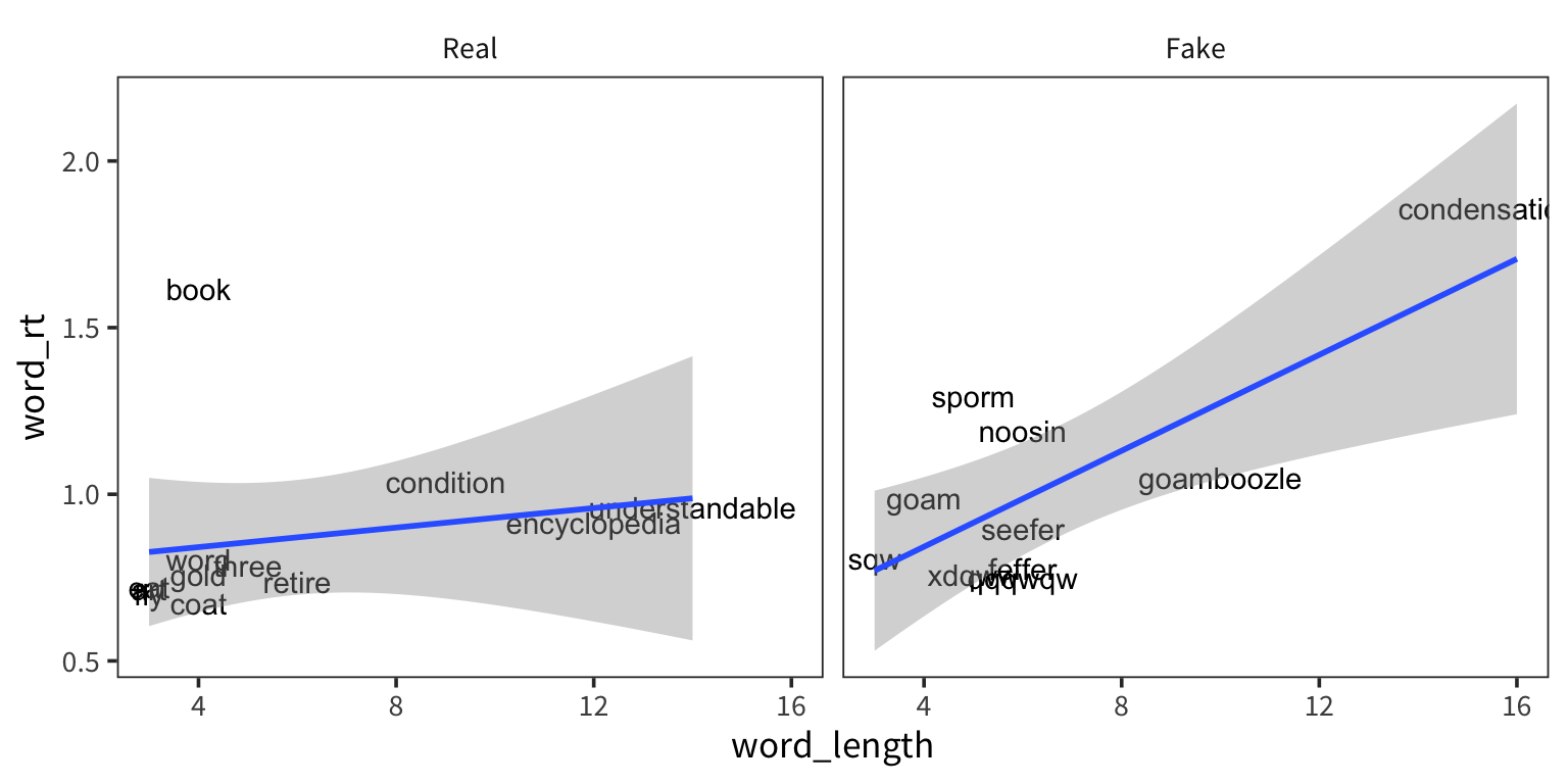
Statistics
Summary statistics
So we’ve been using mean() and sd() already but let’s think some more about what they actually represent and why they’re important.
rt_data <- read_csv("http://web.mit.edu/psycholinglab/www/data/in_lab_rts_2020.csv")
rt_data <- rt_data %>%
  filter(rt < 10, rt > 0.01)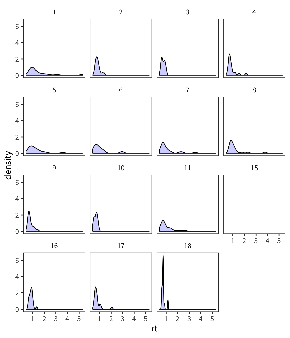
You can see that even in this tiny sample there is quite a bit of variability in terms of how RTs are distributed. And you can sort of see that if you were to try and characterize these distributions, 2 big pieces of information would be central tendency and spread (there’s also things like skew and kurtosis but they’re much less used).
Arithmetic Mean and Median tell us about the central tendency of the data. What about the spread of the data?
First thing that might come to mind? How about the mean distance from the mean?
Let’s try this out by generating a bunch of random numbers now in R from a normal distribution using rnorm().
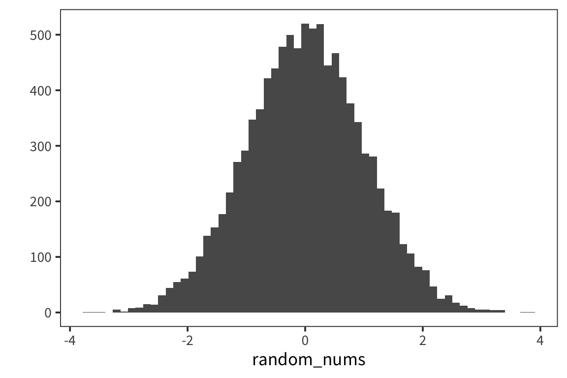
We see our typical Gaussian/bell-curve: most numbers are near zero, and they thin out as you get farther away from zero. We see the mean is zero, or pretty close:
## [1] 0.01624965Let’s look at the mean of mean absolute differences from zero:
## [1] 0.7963574The benefit of the absolute value is to throw away the fact that some things are to the left and others are to the right of the mean. This is called the absolute variance.
But it turns out a similar measure has much nicer mathematical properties down the line. Let’s instead look at the average SQUARED distance to the mean.
## [1] 0.9927534This is called VARIANCE. The square root of variance is called STANDARD DEVIATION or sd. It has a lot of nice properties. You can see one of them here: for Normal-distributed data, the SD is 1.
## [1] 0.9963701We can get the variance and standard deviation using var() and sd()
## [1] 0.9928527## [1] 0.9964199Note that the number you get out of this is SLIGHTLY difference than the one you got out of the formula. We’ll go into why that is later today. Here is the formula which you should use, which gives you the same numbers
## [1] 0.9928527## [1] 0.9964199Now we have measures of central tendency and spread. Remember that we have data that look like this.

For a high-variance subject, something that’s x far from the mean might be equivalent to something that’s y far from the mean for a low-variance subject. We might have similar effects here, just on different scales. We can use mean and standard deviation to roughly put all the data on the same scale. This is called z-scoring.
Writing functions
Before I show you how to compute z-scores, we’ll make a slight detour to learn about writing functions in R.
You’ve seen me use a lot of functions that are either part of base R or part of Hadley Wickham’s tidyverse. But let’s say you want to do something for which no one has yet written a function. What can you do? Make your own function!
Let’s make a silly function, which takes an argument x, and returns x + 1.
## [1] 8You can put any series of expressions you want in a function.
## [1] 8 9 10Functions can take any type of arguments and return any type of values.
Within the functions (or independently) you can use control structures like an IF STATEMENT. This lets you do something IF some expression is TRUE. (similar to if_else())
## [1] "x is greater than 50"We can add an additional clause to this statement, which is something to do OTHERWISE:
compared_to_50 <- function(x) {
  if (x > 50) {
    return("x is greater than 50")
  } else if (x < 50) {
    return("x is less than 50")
  }
}

compared_to_50(100)
## [1] "x is greater than 50"## [1] "x is less than 50"We can chain together lots of if statements…
compared_to_50 <- function(x){
  if (x > 50) {
    return("x is greater than 50")
  } else if (x < 50) {
    return("x is less than 50")
  } else {
    return("x is 50")
  }
}

compared_to_50(100)
## [1] "x is greater than 50"## [1] "x is less than 50"## [1] "x is 50"Try it yourself…
Write a function that takes a vector of numbers as an argument and returns that vector’s mean and standard deviation. (Note that in R functions can only return one object)
Use your function to get the mean and sd of
random_nums.summary_stats <- function(x) { mean_x <- mean(x) sd_x <- sd(x) stats <- c("mean" = mean_x, "sd" = sd_x) return(stats) } summary_stats(random_nums)## mean sd ## 0.01624965 0.99641995
Z-scoring
This says first center your values around the mean value, then divide by SD to stretch out or shrink your space in standardized way. You’re normalizing your scale here so the units are standard deviations: if your z-score is 1, that means that the original datapoint was one standard deviation away from the mean. The idea is that distances in terms of SD are comparable across groups which differ in mean and variance in a way that raw values are not.
## [1] 0.9561173## [1] -6.144535e-17## [1] 0.545665## [1] 1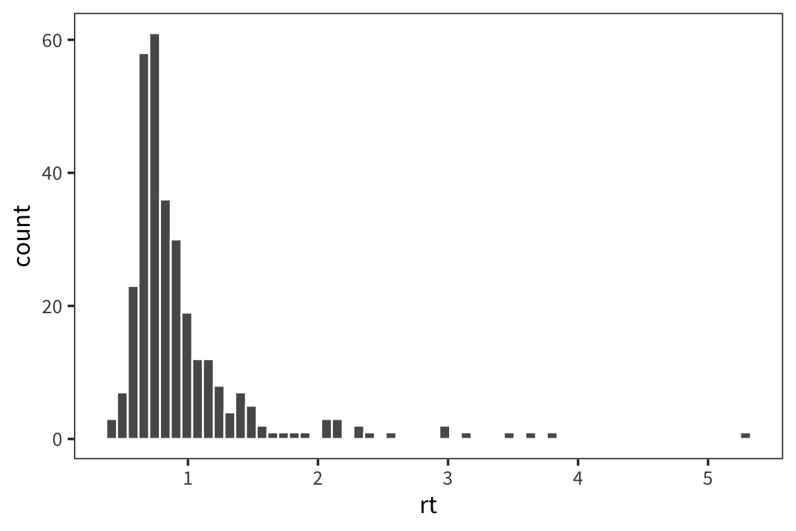
## # A tibble: 15 x 3
## subject mean_rt mean_z_rt
## <dbl> <dbl> <dbl>
## 1 1 1.45 0.897
## 2 2 0.851 -0.194
## 3 3 0.747 -0.383
## 4 4 0.875 -0.150
## 5 5 1.23 0.493
## 6 6 1.05 0.178
## 7 7 1.10 0.264
## 8 8 1.16 0.369
## 9 9 0.797 -0.291
## 10 10 0.686 -0.494
## 11 11 1.01 0.102
## 12 15 1.48 0.960
## 13 16 0.864 -0.168
## 14 17 0.800 -0.286
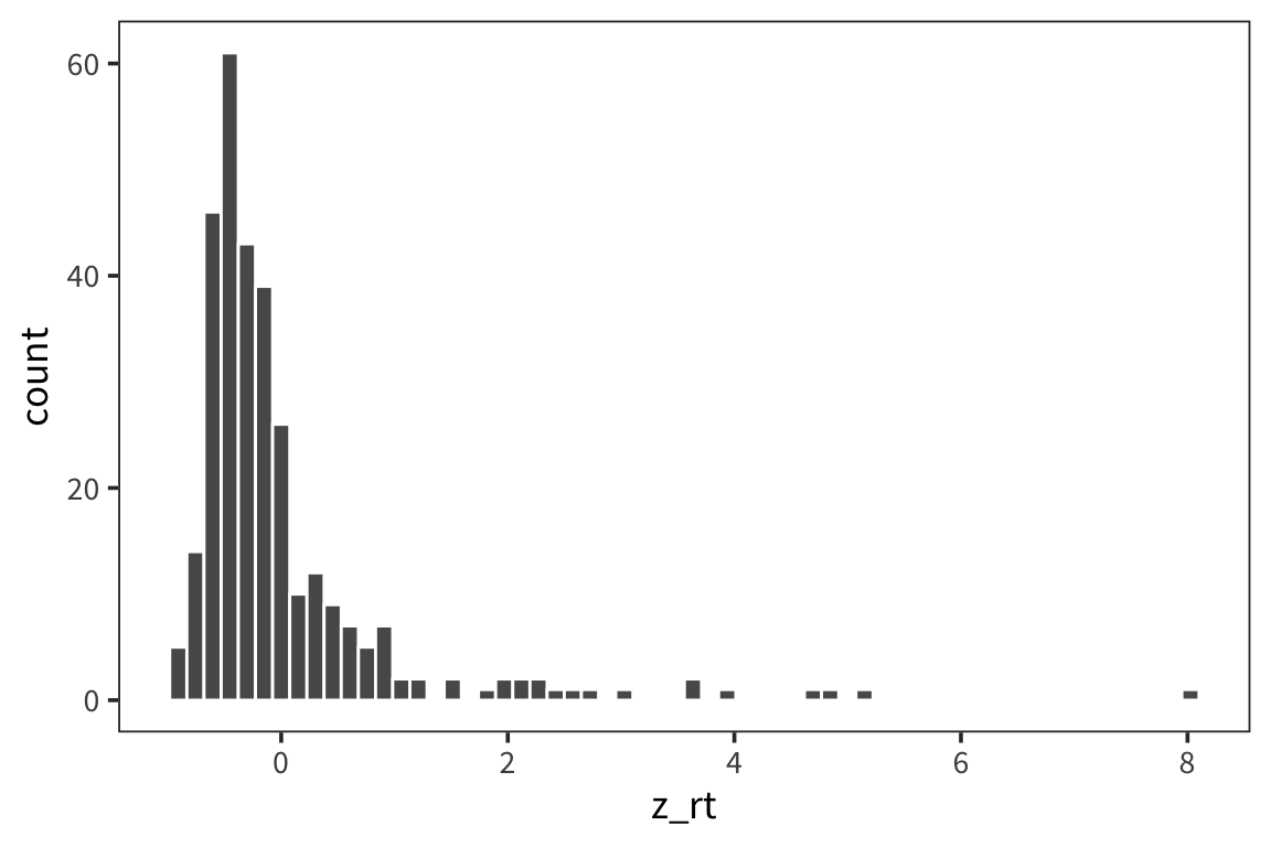
## 15 18 0.755 -0.369You can see that the z-scores are centered on 0 and the shape is a little more gaussian but this doesn’t get rid of outliers.
In general, in the context of the normal distribution we expect about 68% of the datapoints to be within 1 standard deviation of the mean.
So if sd(x) = 10, that means that we expect 68% of the datapoints to be between mean - 10 and mean + 10. We expect 96% of the data to be within 2 standard deviations of the mean, and 99% of the data to be within 3 standard deviations of the mean. These numbers may seem strange and random to you right now but it’ll make more sense as we learn more about the Normal.
The normal distribution
The normal distribution is parameterized by the mean and the standard deviation. When we talk about the parameters of the distribution we’ll call these \(\mu\) and \(\sigma\), rather than mean and sd. These are the parameters you would use to generate a specific distribution (e.g., with rnorm).
# generate 1000 random numbers from a normal distribution with mu 0 and sigma 1
random_nums <- rnorm(1000, 0, 1)
qplot(random_nums, geom = "histogram")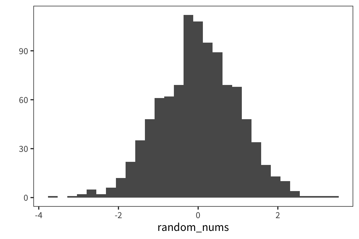
We’ll use mean and sd to refer to the actual values computed from the data that are the result of such a generative process.
## [1] 0.01451242## [1] 0.981466We see the mean is close to \(\mu\), and the sd is close to \(\sigma\) but they are not identical. The mean function provides an ESTIMATE of \(\mu\), and the sd function provides an ESTIMATE of \(\sigma\). (This is why we have to use the corrected sd formula; otherwise it would not be a good estimate of \(\sigma\)).
Let’s look at what happens when we change the parameters of the Normal.
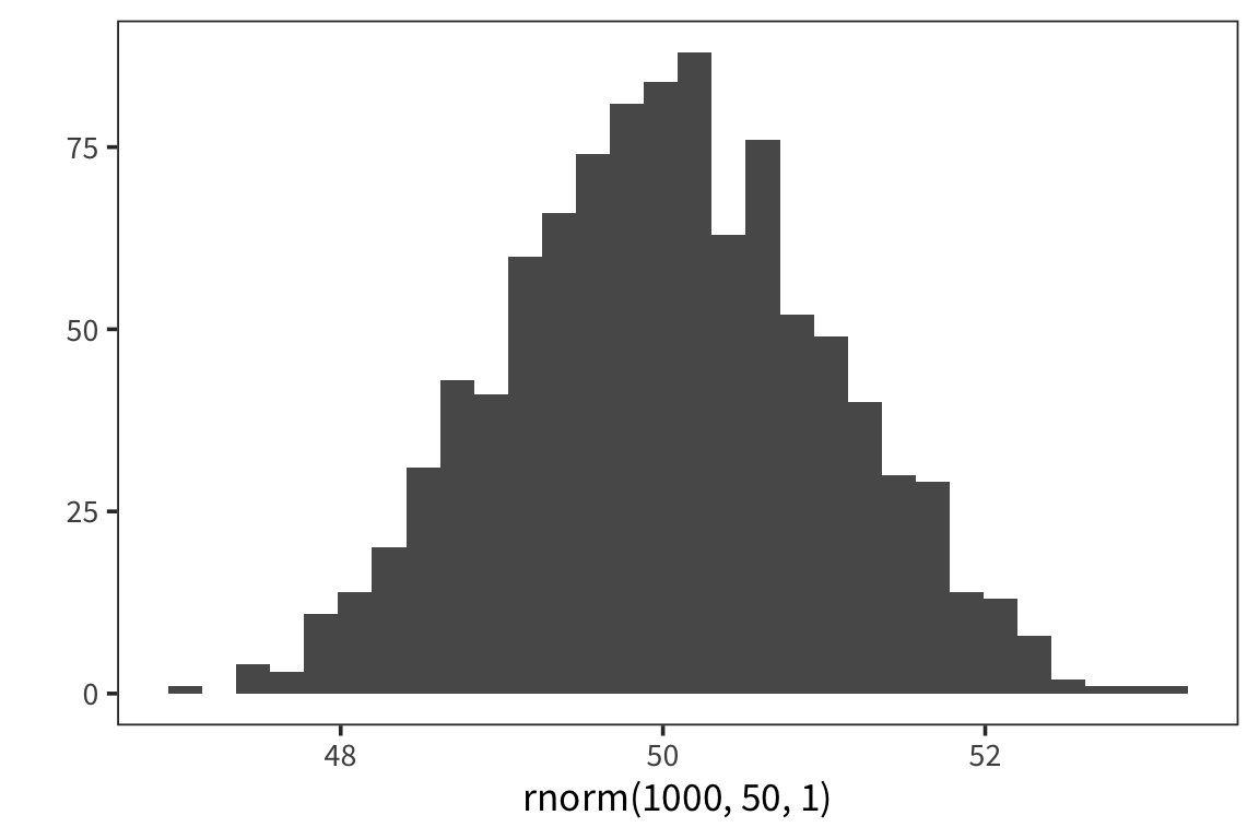
## [1] 49.96973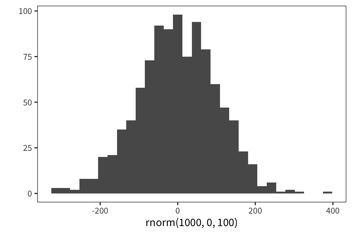
## [1] 103.7158The normal distribution represents a generative process for data. Here it is an R function with two parameters. Say we have lots of datapoints that we know were generated using this function. Now we want to know, what were the values of the two parameters, \(\mu\) and \(\sigma\), which were passed into the function in order to generate this data? We can estimate \(\mu\) using mean(), and \(\sigma\) using sd().
In general, this is a powerful way to think about statistics, and about science in general: we know there is some function that generated the data in front of us, and we want to guess what were the parameters passed into that function? Or what exactly was the function? Recovering these things is the goal of all inference. In the case of data which is normally-distributed, all you need to recover is these two numbers, and you will have a function which can simulate your data.
Let’s see how this works with real data.
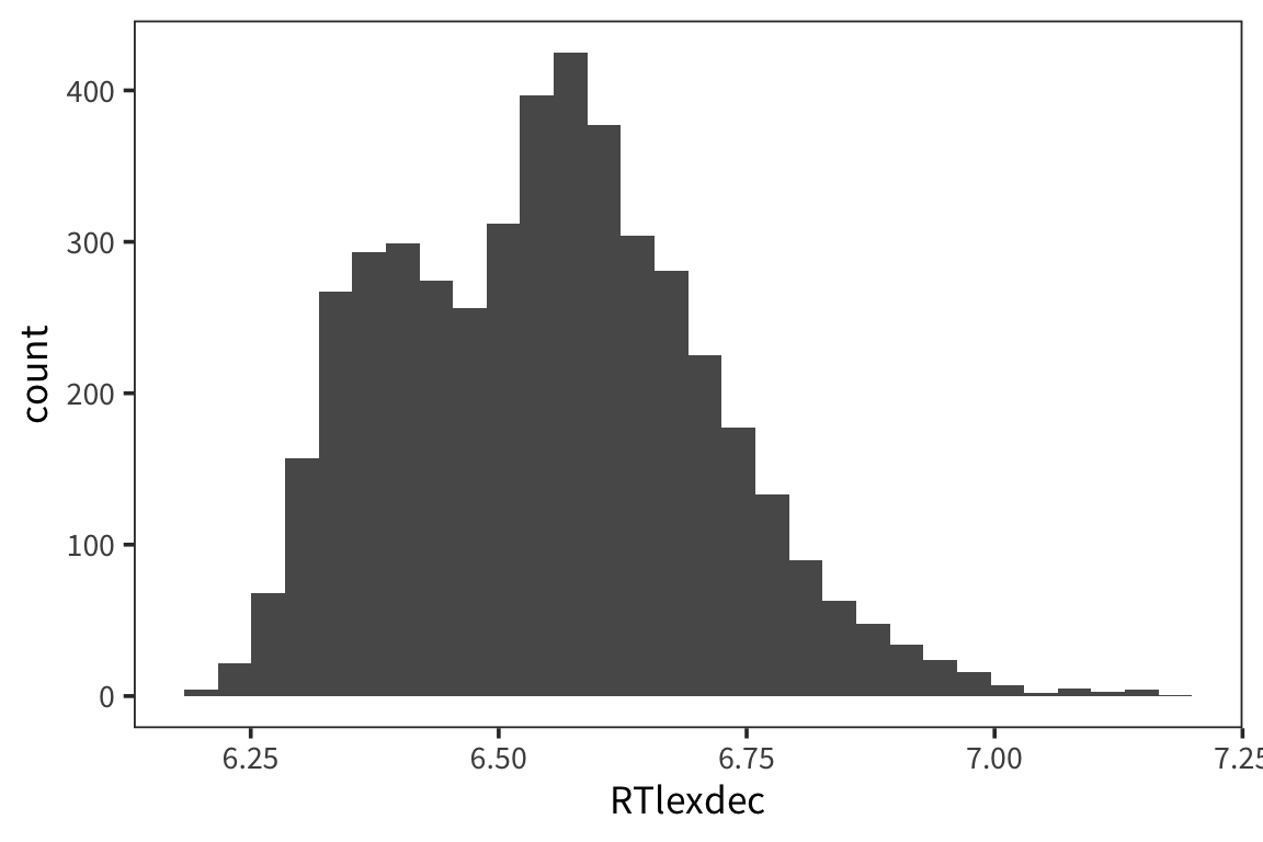
This is somewhat normally distributed. Let’s pretend the data were generated by rnorm, and try to figure out what were the arguments to that function.
## [1] 6.550097## [1] 0.1569188Let’s now draw a bunch of samples from the normal distribution with those parameters, and see if it matches our real data.
fake_rts <- rnorm(nrow(rts), mean(rts$RTlexdec), sd(rts$RTlexdec))
qplot(fake_rts, geom = "histogram")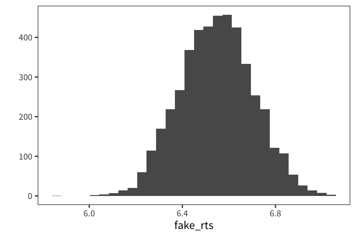
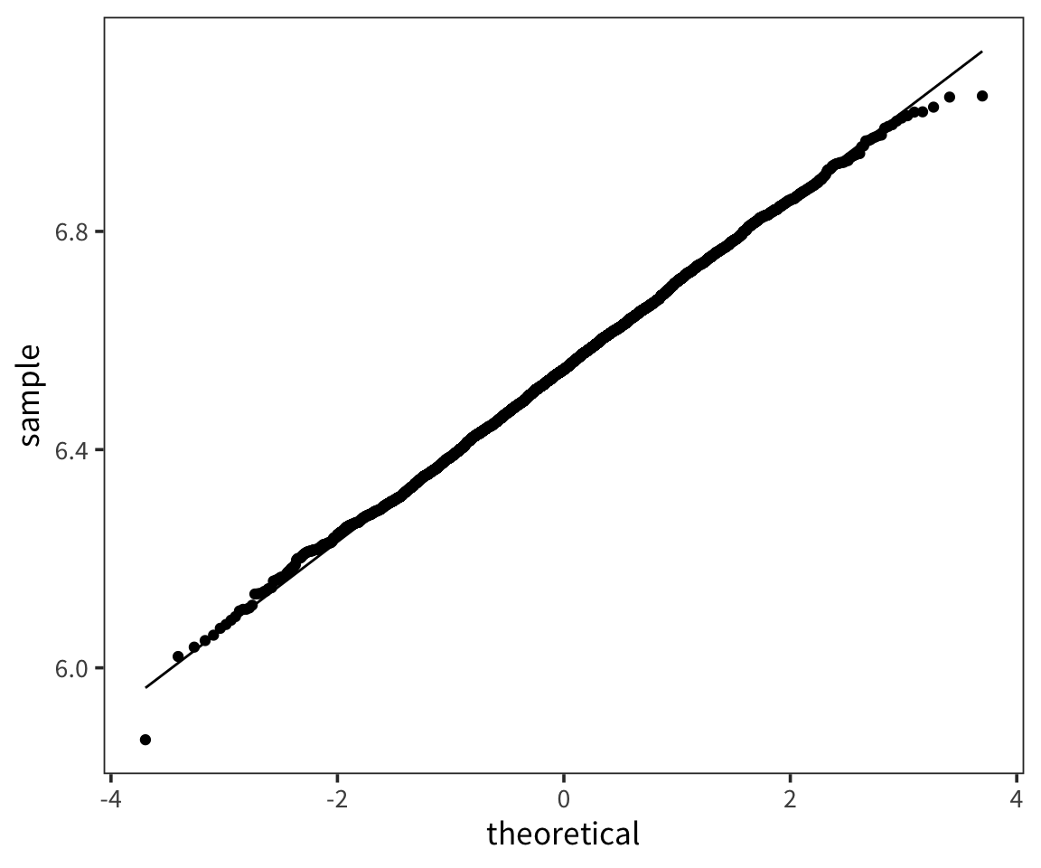
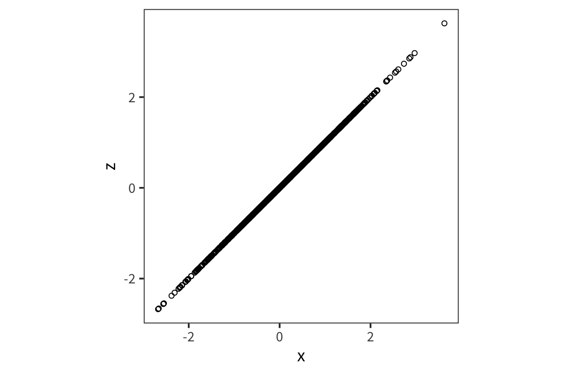
A QQ-plot plots the quantiles of 2 distributions against one another and allows direct comparison. If they are the same distribution, the points will lay on top of the line x=y. By default geom_qq() takes the argument and compares it to the standard normal.

Correlation
Going back to our scatterplots of RTs and word lengths. There was some evidence that there was a relationship there that we could see but what if we want to quantify that? The easiest tool for that is the correlation coefficient.
- The correlation coefficient measures the strength of linear association between two variables.
- It is always between -1 and 1, inclusive, where
- -1 indicates perfect negative relationship
- 0 indicates no relationship
- +1 indicates perfect positive relationship
Pearson’s correlation coefficient: \(r_{xy} =\frac{1}{n-1} \sum_{i=1}^{n}(\frac{x_i-\overline{x}}{s_x})\times(\frac{y_i-\overline{y}}{{s_y}})\)
Note that what’s being multiplied is the z-scored x and y
rt_data <- rt_data %>%
  mutate(word_length = str_length(word))

word_length_scaled <- (rt_data$word_length - mean(rt_data$word_length)) / sd(rt_data$word_length)
rt_scaled <- (rt_data$rt - mean(rt_data$rt)) / sd(rt_data$rt)
pearson_r1 <- sum(word_length_scaled * rt_scaled) / (nrow(rt_data) - 1)
pearson_r2 <- cor(rt_data$word_length, rt_data$rt)
Okay, but what does it mean to multiply all the values together like that? Here is an example of uncorrelated variables.
x <- rnorm(1000)
y <- rnorm(1000)
xy <- data_frame(x, y)
ggplot(xy, aes(x, y)) +
  geom_point(shape = 1) +
  coord_equal()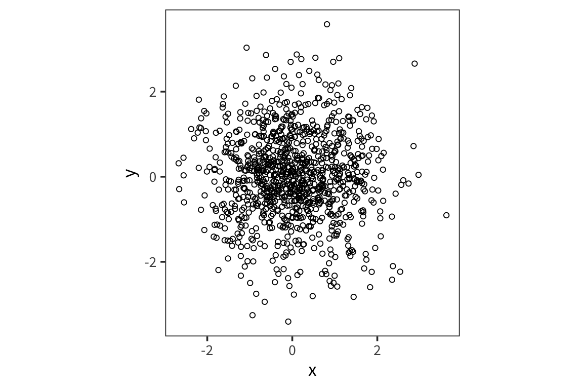
## [1] 0.02373751## [1] 0.02373751On the other hand:
## [1] 1To get a better sense of what different correlation coefficients represent, check out the awesome visualization by Kristoffer Magnuson: http://rpsychologist.com/d3/correlation/.
- try different correlations and see the effect of moving outliers
- try different sample sizes and see the effect of outliers
To sharpen your intuitions about correlation (read: have fun with stats!), play Guess the Correlation: http://guessthecorrelation.com/.
Data wrangling (tidyr)
So far we’ve mostly dealt with data that’s neatly organized into a format that is easy for us to manipulate with things like filter() and mutate(). In general, this kind of tidy format makes things easier: one row for every trial for each subject. Often data will not be organized so neatly from the get-go and you will have to do some serious data wrangling to get it into the format you want. In particular, you’ll see that Amazon Mechanical Turk output is often in wide format. For these purposes you will need to know functions like pivot_longer(), pivot_wider(), and separate().
First let’s set up our workspace and read in some data files. These contain data from a study of lexical decision latencies in beginning readers (8 year-old Dutch children). This is available as the beginningReaders dataset from languageR but here I’ve split it up into separate datasets so that we can see how we could put it back together.
data_source <- "http://web.mit.edu/psycholinglab/www/data/"
word_data <- read_csv(file.path(data_source, "word_data.csv"))
subject_data <- read_csv(file.path(data_source, "subject_data.csv"))
logRT_data <- read_csv(file.path(data_source, "logRT_data.csv"))
Let’s look at these data:
## # A tibble: 736 x 3
##    Word     metric         v
##    <chr>    <chr>      <dbl>
##  1 avontuur OrthLength     8
##  2 baden    OrthLength     5
##  3 balkon   OrthLength     6
##  4 band     OrthLength     4
##  5 barsten  OrthLength     7
##  6 beek     OrthLength     4
##  7 beker    OrthLength     5
##  8 beton    OrthLength     5
##  9 beven    OrthLength     5
## 10 bieden   OrthLength     6
## # … with 726 more rows
Here we see that we have a list of words and a series of metrics for each word with an associated value.
## # A tibble: 59 x 2
##    Subject ReadingScore
##    <chr>          <dbl>
##  1 S28               39
##  2 S40               34
##  3 S37               61
##  4 S65               66
##  5 S54               41
##  6 S43               23
##  7 S34               28
##  8 S47               60
##  9 S61               87
## 10 S39               39
## # … with 49 more rows
Here we have a reading score for each subject.
## # A tibble: 59 x 185
##    Subject avontuur baden balkon band  barsten beek  beker beton beven
##    <chr>   <chr>    <chr> <chr>  <chr> <chr>   <chr> <chr> <chr> <chr>
##  1 S10     407t8.0… 398t… 133t6… 98t7… 237t7.… 363t… 186t… <NA>  38t6…
##  2 S12     155t7.6… 311t… 386t7… 108t… 20t7.0… 394t… 272t… <NA>  99t7…
##  3 S13     352t7.4… 183t… <NA>   414t… 508t7.… 86t7… 230t… 283t… 425t…
##  4 S14     94t7.76… <NA>  <NA>   442t… <NA>    <NA>  <NA>  511t… 494t…
##  5 S15     70t7.33… 78t7… 345t7… 378t… 244t7.… 114t… 293t… 459t… 438t…
##  6 S16     194t6.3… 374t… <NA>   146t… <NA>    <NA>  315t… <NA>  <NA>
##  7 S18     358t7.5… 165t… 83t7.… 415t… <NA>    76t7… 214t… <NA>  425t…
##  8 S2      87t7.50… 95t7… 373t6… 415t… 263t7.… 132t… 315t… <NA>  480t…
##  9 S20     <NA>     <NA>  401t7… 442t… <NA>    159t… 337t… 511t… <NA>
## 10 S21     400t7.2… <NA>  133t7… 101t… 230t7.… 360t… 182t… 19t7… 43t7…
## # … with 49 more rows, and 175 more variables: bieden <chr>,
## #   blaffen <chr>, blinken <chr>, bocht <chr>, bonzen <chr>,
## #   boodschap <chr>, bord <chr>, broek <chr>, broer <chr>, brok <chr>,
## #   brullen <chr>, buit <chr>, bukken <chr>, cent <chr>, deken <chr>,
## #   douche <chr>, durven <chr>, dwingen <chr>, echo <chr>, emmer <chr>,
## #   flitsen <chr>, fluisteren <chr>, fruit <chr>, gapen <chr>,
## #   garage <chr>, giechelen <chr>, gieten <chr>, gillen <chr>,
## #   glinsteren <chr>, gloeien <chr>, gluren <chr>, graan <chr>,
## #   grap <chr>, grijns <chr>, grijnzen <chr>, grinniken <chr>,
## #   groeten <chr>, grommen <chr>, grot <chr>, hijgen <chr>, hijsen <chr>,
## #   horizon <chr>, horloge <chr>, insekt <chr>, jagen <chr>,
## #   juichen <chr>, kanon <chr>, karton <chr>, karwei <chr>, kerel <chr>,
## #   ketel <chr>, kilo <chr>, kin <chr>, klagen <chr>, klant <chr>,
## #   knagen <chr>, kneden <chr>, knielen <chr>, knipperen <chr>,
## #   knol <chr>, koffer <chr>, koning <chr>, koren <chr>, korst <chr>,
## #   kraag <chr>, kreunen <chr>, krijsen <chr>, krimpen <chr>, kudde <chr>,
## #   kus <chr>, ladder <chr>, laden <chr>, lawaai <chr>, leunen <chr>,
## #   liegen <chr>, lijden <chr>, liter <chr>, loeren <chr>, manier <chr>,
## #   matras <chr>, matroos <chr>, melden <chr>, mengen <chr>,
## #   metselen <chr>, minuut <chr>, mompelen <chr>, mouw <chr>, mus <chr>,
## #   muts <chr>, neef <chr>, ober <chr>, oever <chr>, oom <chr>,
## #   paradijs <chr>, parfum <chr>, park <chr>, pet <chr>, piepen <chr>,
## #   pijl <chr>, piloot <chr>, …
Here we have 1 column for subject and then a column for each word they saw. The cells contain a weird value or NA. The weird value is a combination of the trial number and log response time (separated by the “t”).
So ultimately what we want is 1 big dataset where we have 1 subject column, 1 trial number column, 1 word column and then 1 column for each of value, logRT, OrthLenght, LogFrequency, etc…
Tidying
So let’s start by making each individual dataframe tidier.
We want word_data to go from 1 “metric” column to a column for each of the 4 metrics. So you can think of this as making the data wider.
subject_data is very simple so we can leave it for now.
For logRT_data, we want to do the opposite: we want to have a column for words and for trial numbers and logRTs. So we want to make the data longer by making all the individual word columns into 2 columns the word and that weird value that’s currently in the cells.
logRT_data_long <- logRT_data %>%
  pivot_longer(names_to = "Word", values_to = "weird_value", cols = -Subject)
Okay, now we want to separate this weird value into 2 columns, Trial and LogRT
Joins
So now we’re ready to join all 3 of these dataframes together.
First, let’s combine the logRTs with the subjects’ reading scores. So we want there to be the same reading score across multiple rows because the reading score is the same for a subject no matter which trial.
subject_plus_logRT_data <- left_join(x = logRT_data_tidy,
                                     y = subject_data,
                                     by = "Subject")
subject_plus_logRT_data
## # A tibble: 10,856 x 5
## Subject Word Trial LogRT ReadingScore
## <chr> <chr> <chr> <dbl> <dbl>
## 1 S10 avontuur 407 8.06 59
## 2 S10 baden 398 7.93 59
## 3 S10 balkon 133 6.84 59
## 4 S10 band 98 7.20 59
## 5 S10 barsten 237 7.72 59
## 6 S10 beek 363 7.47 59
## 7 S10 beker 186 7.46 59
## 8 S10 beton <NA> NA 59
## 9 S10 beven 38 6.91 59
## 10 S10 bieden 66 7.85 59
## # … with 10,846 more rowsNote that there is only 1 “Subject” column in the resulting data file.
Now let’s combine this new dataframe with the word_data. Here we expect repetition within a word but not a subject since the words LogFrequency (for example) will not differ depending on which subject is reading it.
## # A tibble: 10,856 x 9
##    Subject Word  Trial LogRT ReadingScore OrthLength LogFrequency
##    <chr>   <chr> <chr> <dbl>        <dbl>      <dbl>        <dbl>
##  1 S10     avon… 407    8.06           59          8         4.39
##  2 S12     avon… 155    7.66           76          8         4.39
##  3 S13     avon… 352    7.41           54          8         4.39
##  4 S14     avon… 94     7.76           18          8         4.39
##  5 S15     avon… 70     7.33           50          8         4.39
##  6 S16     avon… 194    6.36           10          8         4.39
##  7 S18     avon… 358    7.60           40          8         4.39
##  8 S2      avon… 87     7.50           50          8         4.39
##  9 S20     avon… <NA>  NA              19          8         4.39
## 10 S21     avon… 400    7.27           50          8         4.39
## # … with 10,846 more rows, and 2 more variables: LogFamilySize <dbl>,
## #   ProportionOfErrors <dbl>
Note there are some NA values because we have some words that weren’t experienced by all the subjects. We can get rid of those. But be very careful with this. A lot of NAs in your data where you weren’t expecting them are often a sign that you made an error somewhere in your data wrangling.
Now if you want you can compare this to the first 8 columns of the beginningReaders dataset from languageR.
So now that we have some data in a tidy form we can start looking for patterns…
all_data %>%
  group_by(ReadingScore) %>%
  summarise(mean_logRT = mean(LogRT)) %>%
  ggplot(aes(x = ReadingScore, y = mean_logRT)) +
    geom_point(shape = 1) +
    geom_smooth(method = "lm")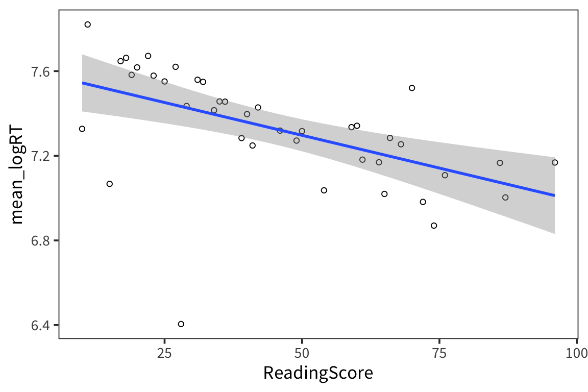
So it looks like there is a relationship between subjects’ reading scores and RTs
all_data %>%
  group_by(LogFamilySize) %>%
  summarise(mean_logRT = mean(LogRT)) %>%
  ggplot(aes(x = LogFamilySize, y = mean_logRT)) +
    geom_point(shape = 1)  +
    geom_smooth(method = "lm")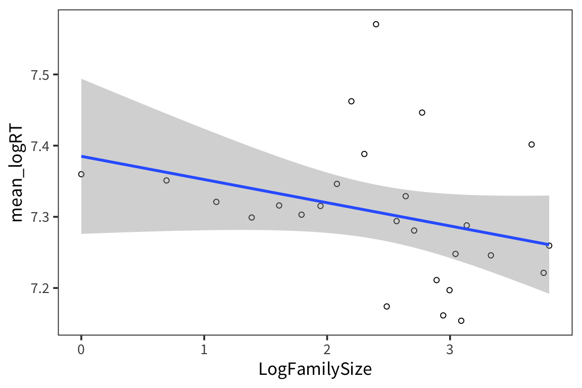
Creating data frames
There are several different ways to create dataframes from scratch. tibble() does it by column, while tribble() does it by row.
## # A tibble: 3 x 2
##   subject height
##   <chr>    <dbl>
## 1 Alice       66
## 2 Bob         63
## 3 Charlie 72## # A tibble: 3 x 2
## subject height
## <chr> <dbl>
## 1 Alice 66
## 2 Bob 63
## 3 Charlie 72Try it yourself…
- Read in the data we collected in lab on the first day (
in_lab_rts_2020.csv) asrt_data. - Make a new dataset
rt_data_wide, which a) doesn’t contain the “time” column and b) in which there’s one column for each word. HINT: you may want to firstunite()2 columns. - Now take
rt_data_wideand make a new dataset,rt_data_long, which has a column for word and a column for trial. - Create a new dataframe
word_typesthat has a row for every word inrt_dataand columns for the word and for indicating whether the word is real or fake. - Join
rt_dataandword_typestogether intort_data_coded. - How many real and fake words were there in the experiment? How many real and fake trials were there?